Poteri della matrice -

In questa pagina vedremo come fare le potenze delle matrici. Troverai anche esempi ed esercizi di potenze di matrici risolti passo passo che ti aiuteranno a capirlo perfettamente. Imparerai anche cos’è l’ennesima potenza di una matrice e come trovarla.

Come si calcola la potenza di una matrice?

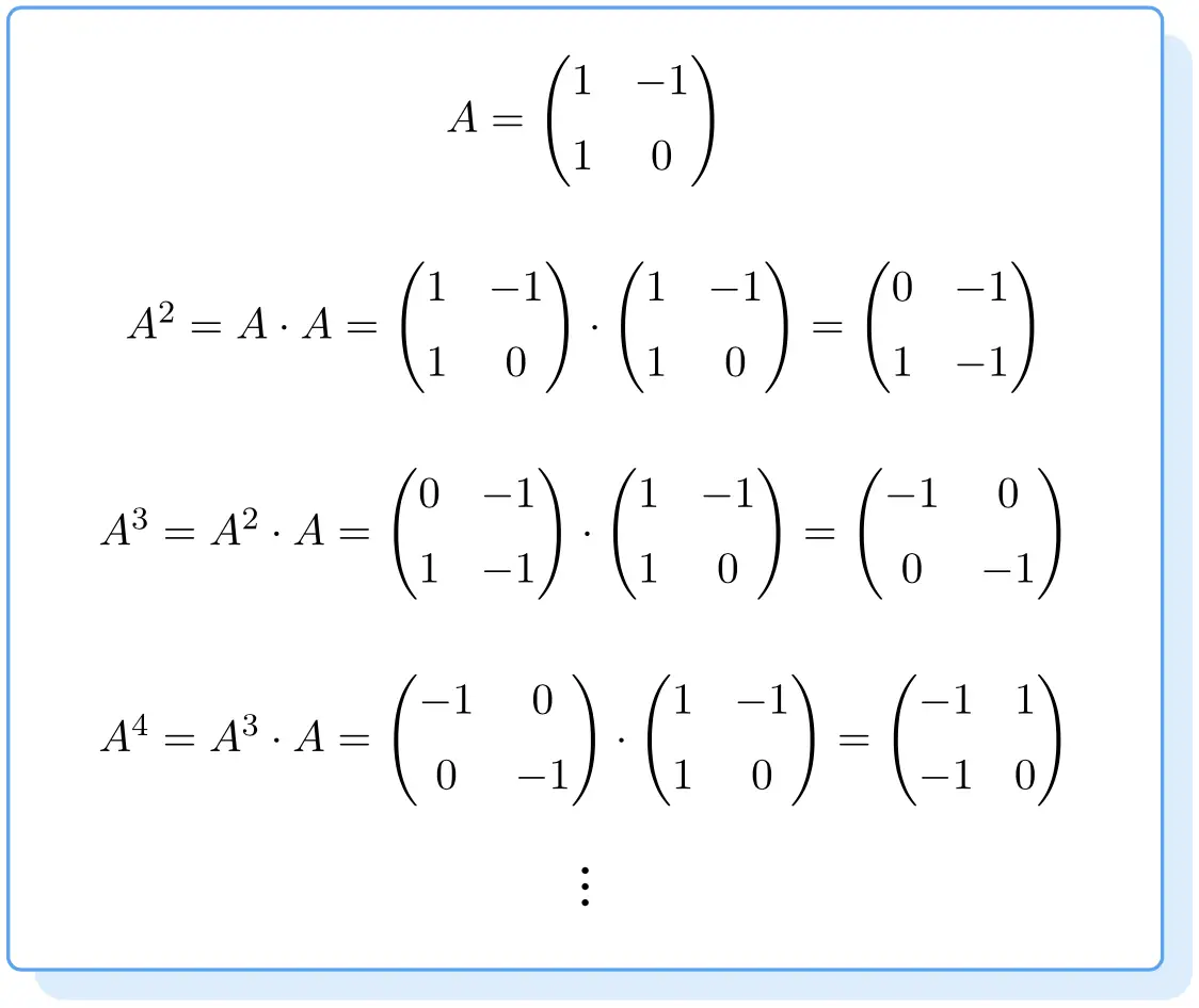
Per calcolare la potenza di una matrice , devi moltiplicare la matrice per se stessa tante volte quanto dice l’esponente. Per esempio:

$A^4 = A \cdot A \cdot A \cdot A$

Pertanto, per ottenere la potenza di una matrice, è necessario sapere come risolvere la moltiplicazione di matrici . Altrimenti non è possibile calcolare una matrice di potenze.

Esempio di calcolo della potenza di una matrice:

Pertanto, la potenza di una matrice quadrata si calcola moltiplicando la matrice per se stessa. Allo stesso modo, una matrice cubica è uguale alla matrice quadrata della matrice stessa. Allo stesso modo, per trovare la potenza di una matrice elevata a quattro, la matrice elevata a tre deve essere moltiplicata per la matrice stessa. E così via.

C’è un’importante proprietà della potenza di una matrice che dovresti conoscere: la potenza di una matrice può essere calcolata solo quando è quadrata , cioè quando ha lo stesso numero di righe e colonne.

Qual è la potenza n di una matrice?

L’ ennesima potenza di una matrice è un’espressione che ci permette di calcolare facilmente qualsiasi potenza di una matrice.

Spesso le potenze delle matrici seguono uno schema . Pertanto, se riusciamo a decifrare la sequenza che seguono, saremo in grado di calcolare qualsiasi potenza senza dover fare tutte le moltiplicazioni.

Ciò significa che possiamo trovare una formula che ci dia l’ennesima potenza di una matrice senza dover calcolare tutte le potenze.

Suggerimenti per scoprire lo schema seguito dai poteri:

La parità dell’esponente . Può darsi che i poteri pari siano in un modo e i poteri dispari nell’altro.
Variazione dei segni. Ad esempio, potrebbe essere che gli elementi delle potenze pari siano positivi e gli elementi delle potenze dispari siano negativi o viceversa.
Ripetizione: se la stessa matrice viene ripetuta ogni certo numero di potenze oppure no.
Dobbiamo anche vedere se esiste una relazione tra l’esponente e gli elementi della matrice.

Esempio di calcolo della potenza n di una matrice:

Essere
$A$

la seguente matrice, calcolare

$A^n$

E

$A^{100}$

.

$\displaystyle A = \begin{pmatrix} 1 & 1 \\[1.1ex] 1 & 1 \end{pmatrix}$

Per prima cosa calcoleremo diverse potenze della matrice

$A$

, per cercare di indovinare lo schema seguito dai poteri. Quindi calcoliamo

$A^2$

$A^3$

$A^4$

$A^5:$

esercizio risolto passo passo sulle potenze delle matrici 2x2

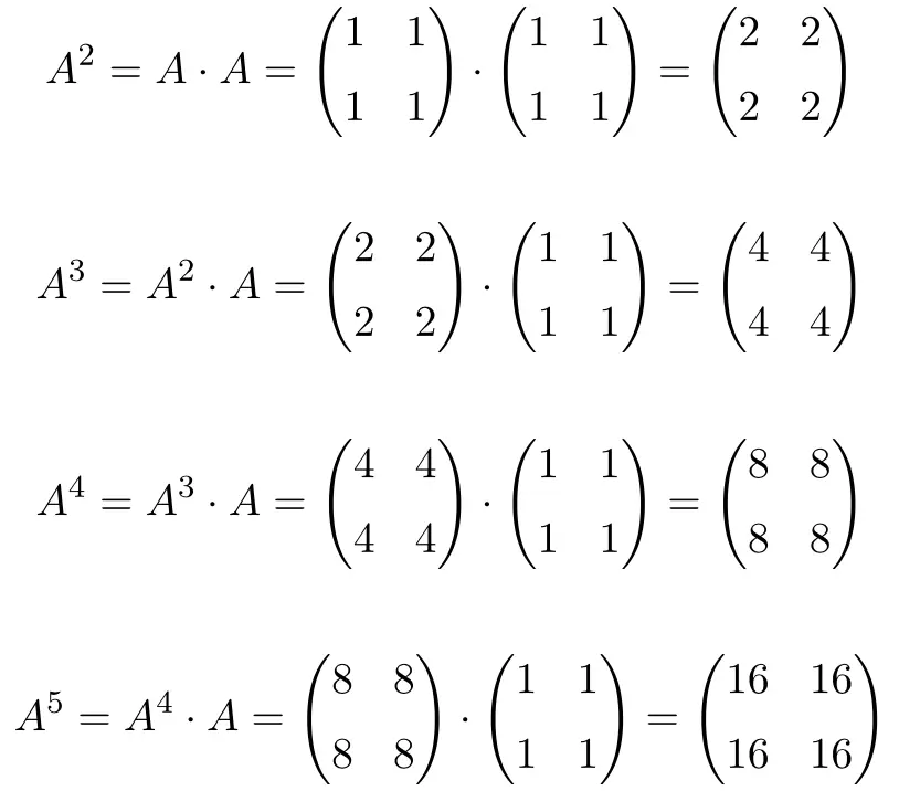
Quando si calcola fino a

$A^5$

, vediamo che le potenze della matrice

$A$

Seguono uno schema: per ogni aumento di potenza, il risultato viene moltiplicato per 2. Pertanto, tutte le matrici sono potenze di 2:

$\displaystyle A^2= \begin{pmatrix} 2 & 2 \\[1.1ex] 2 & 2 \end{pmatrix} =\begin{pmatrix} 2^1 & 2^1 \\[1.1ex] 2^1 & 2^1 \end{pmatrix}$

$\displaystyle A^3= \begin{pmatrix} 4 & 4 \\[1.1ex] 4 & 4 \end{pmatrix}=\begin{pmatrix} 2^2 & 2^2 \\[1.1ex] 2^2 & 2^2 \end{pmatrix}$

$\displaystyle A^4= \begin{pmatrix} 8 & 8 \\[1.1ex] 8 & 8 \end{pmatrix}=\begin{pmatrix} 2^3 & 2^3 \\[1.1ex] 2^3 & 2^3 \end{pmatrix}$

$\displaystyle A^5= \begin{pmatrix} 16 & 16 \\[1.1ex] 16 & 16 \end{pmatrix}=\begin{pmatrix} 2^4 & 2^4 \\[1.1ex] 2^4 & 2^4 \end{pmatrix}$

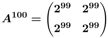
Possiamo quindi derivare la formula per l’ ennesima potenza della matrice

$A:$

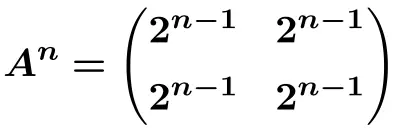
E da questa formula possiamo calcolare

$A^{100}:$

esercizio risolto passo passo potenza di una matrice 2x2

Risolti i problemi di alimentazione della matrice

Esercizio 1

Consideriamo la seguente matrice di dimensione 2×2:

$\displaystyle A=\begin{pmatrix} 1 & 2 \\[1.1ex] -1 & 1 \end{pmatrix}$

Calcolare:

$\displaystyle A^4$

vedi soluzione

Per calcolare la potenza di una matrice, devi moltiplicare la matrice una per una. Pertanto, calcoliamo prima

$\displaystyle A^2 :$

$\displaystyle A^2= A \cdot A = \begin{pmatrix} 1 & 2 \\[1.1ex] -1 & 1 \end{pmatrix} \cdot \begin{pmatrix} 1 & 2 \\[1.1ex] -1 & 1 \end{pmatrix} = \begin{pmatrix} -1 & 4 \\[1.1ex] -2 & -1\end{pmatrix}$

Ora calcoliamo

$\displaystyle A^3 :$

$\displaystyle A^3= A^2 \cdot A = \begin{pmatrix} -1 & 4 \\[1.1ex] -2 & -1 \end{pmatrix} \cdot \begin{pmatrix} 1 & 2 \\[1.1ex] -1 & 1 \end{pmatrix} =\begin{pmatrix} -5 & 2 \\[1.1ex] -1 & -5 \end{pmatrix}$

E infine calcoliamo

$\displaystyle A^4 :$

$\displaystyle A^4= A^3 \cdot A = \begin{pmatrix} -5 & 2 \\[1.1ex] -1 & -5 \end{pmatrix} \cdot \begin{pmatrix} 1 & 2 \\[1.1ex] -1 & 1 \end{pmatrix} = \begin{pmatrix} \bm{-7} & \bm{-8} \\[1.1ex] \bm{4} & \bm{-7} \end{pmatrix}$

Esercizio 2

Consideriamo la seguente matrice di ordine 2:

$\displaystyle A=\begin{pmatrix} 1 & 0 \\[1.1ex] 0 & 3 \end{pmatrix}$

Calcolare:

$\displaystyle A^{35}$

vedi soluzione

$\displaystyle A^{35}$

è un potere troppo grande per essere calcolato a mano, quindi i poteri della matrice devono seguire uno schema. Quindi calcoliamo

$\displaystyle A^5$

per cercare di capire la sequenza che seguono:

$\displaystyle A^2= A \cdot A = \begin{pmatrix} 1 & 0 \\[1.1ex] 0 & 3 \end{pmatrix} \cdot \begin{pmatrix}1 & 0 \\[1.1ex] 0 & 3 \end{pmatrix} = \begin{pmatrix} 1 & 0 \\[1.1ex] 0 & 9 \end{pmatrix}$

$\displaystyle A^3= A^2 \cdot A = \begin{pmatrix} 1 & 0 \\[1.1ex] 0 & 9 \end{pmatrix} \cdot \begin{pmatrix}1 & 0 \\[1.1ex] 0 & 3 \end{pmatrix} = \begin{pmatrix} 1 & 0 \\[1.1ex] 0 & 27 \end{pmatrix}$

$\displaystyle A^4= A^3 \cdot A = \begin{pmatrix}1 & 0 \\[1.1ex] 0 & 27 \end{pmatrix} \cdot \begin{pmatrix}1 & 0 \\[1.1ex] 0 & 3 \end{pmatrix} = \begin{pmatrix} 1 & 0 \\[1.1ex] 0 & 81 \end{pmatrix}$

$\displaystyle A^5= A^4 \cdot A = \begin{pmatrix}1 & 0 \\[1.1ex] 0 & 81 \end{pmatrix} \cdot \begin{pmatrix}1 & 0 \\[1.1ex] 0 & 3 \end{pmatrix} = \begin{pmatrix} 1 & 0 \\[1.1ex] 0 & 243 \end{pmatrix}$

In questo modo possiamo vedere lo schema che seguono le potenze: ad ogni potenza tutti i numeri rimangono gli stessi, tranne l’elemento nella seconda colonna della seconda riga, che viene moltiplicato per 3. Pertanto, tutti i numeri rimangono sempre gli stessi. e l’ultimo elemento è una potenza di 3:

$\displaystyle A=\begin{pmatrix} 1 & 0 \\[1.1ex] 0 & 3 \end{pmatrix}=\begin{pmatrix} 1 & 0 \\[1.1ex] 0 & 3^1 \end{pmatrix}$

$\displaystyle A^2=\begin{pmatrix} 1 & 0 \\[1.1ex] 0 & 9 \end{pmatrix}=\begin{pmatrix} 1 & 0 \\[1.1ex] 0 & 3^2 \end{pmatrix}$

$\displaystyle A^3=\begin{pmatrix} 1 & 0 \\[1.1ex] 0 & 27 \end{pmatrix}=\begin{pmatrix} 1 & 0 \\[1.1ex] 0 & 3^3 \end{pmatrix}$

$\displaystyle A^4=\begin{pmatrix} 1 & 0 \\[1.1ex] 0 & 81 \end{pmatrix}=\begin{pmatrix} 1 & 0 \\[1.1ex] 0 & 3^4 \end{pmatrix}$

$\displaystyle A^5=\begin{pmatrix} 1 & 0 \\[1.1ex] 0 & 243 \end{pmatrix}=\begin{pmatrix} 1 & 0 \\[1.1ex] 0 & 3^5 \end{pmatrix}$

Quindi la formula per l’ennesima potenza della matrice

$\displaystyle A$

Est:

$\displaystyle A^n=\begin{pmatrix} 1 & 0 \\[1.1ex] 0 & 3^n\end{pmatrix}$

E da questa formula possiamo calcolare

$\displaystyle A^{35}:$

$\displaystyle\bm{A^{35}=}\begin{pmatrix} \bm{1} & \bm{0} \\[1.1ex] \bm{0} & \bm{3^{35}}\end{pmatrix}$

Esercizio 3

Consideriamo la seguente matrice 3×3:

$\displaystyle A=\begin{pmatrix} 1 & \frac{1}{5} & \frac{1}{5} \\[1.1ex] 0 & 1 & 0 \\[1.1ex] 0 & 0 & 1 \end{pmatrix}$

Calcolare:

$\displaystyle A^{100}$

vedi soluzione

$\displaystyle A^{100}$

è un potere troppo grande per essere calcolato a mano, quindi i poteri della matrice devono seguire uno schema. Quindi calcoliamo

$\displaystyle A^5$

per cercare di capire la sequenza che seguono:

$\displaystyle A^2= A \cdot A = \begin{pmatrix} 1 & \frac{1}{5} & \frac{1}{5} \\[1.1ex] 0 & 1 & 0 \\[1.1ex] 0 & 0 & 1 \end{pmatrix} \cdot \begin{pmatrix}1 & \frac{1}{5} & \frac{1}{5} \\[1.1ex] 0 & 1 & 0 \\[1.1ex] 0 & 0 & 1 \end{pmatrix} = \begin{pmatrix} 1 & \frac{2}{5} & \frac{2}{5} \\[1.1ex] 0 & 1 & 0 \\[1.1ex] 0 & 0 & 1 \end{pmatrix}$

$\displaystyle A^3= A^2 \cdot A = \begin{pmatrix} 1 & \frac{2}{5} & \frac{2}{5} \\[1.1ex] 0 & 1 & 0 \\[1.1ex] 0 & 0 & 1\end{pmatrix} \cdot \begin{pmatrix}1 & \frac{1}{5} & \frac{1}{5} \\[1.1ex] 0 & 1 & 0 \\[1.1ex] 0 & 0 & 1 \end{pmatrix} = \begin{pmatrix} 1 & \frac{3}{5} & \frac{3}{5} \\[1.1ex] 0 & 1 & 0 \\[1.1ex] 0 & 0 & 1 \end{pmatrix}$

$\displaystyle A^4= A^3 \cdot A = \begin{pmatrix} 1 & \frac{3}{5} & \frac{3}{5} \\[1.1ex] 0 & 1 & 0 \\[1.1ex] 0 & 0 & 1\end{pmatrix} \cdot \begin{pmatrix}1 & \frac{1}{5} & \frac{1}{5} \\[1.1ex] 0 & 1 & 0 \\[1.1ex] 0 & 0 & 1 \end{pmatrix} = \begin{pmatrix} 1 & \frac{4}{5} & \frac{4}{5} \\[1.1ex] 0 & 1 & 0 \\[1.1ex] 0 & 0 & 1 \end{pmatrix}$

$\displaystyle A^5= A^4 \cdot A = \begin{pmatrix} 1 & \frac{4}{5} & \frac{4}{5} \\[1.1ex] 0 & 1 & 0 \\[1.1ex] 0 & 0 & 1\end{pmatrix} \cdot \begin{pmatrix}1 & \frac{1}{5} & \frac{1}{5} \\[1.1ex] 0 & 1 & 0 \\[1.1ex] 0 & 0 & 1 \end{pmatrix} = \begin{pmatrix} 1 & \frac{5}{5} & \frac{5}{5} \\[1.1ex] 0 & 1 & 0 \\[1.1ex] 0 & 0 & 1 \end{pmatrix}$

In questo modo possiamo vedere lo schema che seguono le potenze: ad ogni potenza, tutti i numeri rimangono gli stessi, tranne le frazioni, che aumentano di uno al numeratore:

$\displaystyle A=\begin{pmatrix} 1 & \frac{1}{5} & \frac{1}{5} \\[1.1ex] 0 & 1 & 0 \\[1.1ex] 0 & 0 & 1 \end{pmatrix}$

$\displaystyle A^2= \begin{pmatrix} 1 & \frac{2}{5} & \frac{2}{5} \\[1.1ex] 0 & 1 & 0 \\[1.1ex] 0 & 0 & 1 \end{pmatrix}$

$\displaystyle A^3= \begin{pmatrix} 1 & \frac{3}{5} & \frac{3}{5} \\[1.1ex] 0 & 1 & 0 \\[1.1ex] 0 & 0 & 1 \end{pmatrix}$

$\displaystyle A^4= \begin{pmatrix} 1 & \frac{4}{5} & \frac{4}{5} \\[1.1ex] 0 & 1 & 0 \\[1.1ex] 0 & 0 & 1 \end{pmatrix}$

$\displaystyle A^5= \begin{pmatrix} 1 & \frac{5}{5} & \frac{5}{5} \\[1.1ex] 0 & 1 & 0 \\[1.1ex] 0 & 0 & 1 \end{pmatrix}$

Quindi la formula per la potenza dell’ennesima matrice

$\displaystyle A$

Est:

$\displaystyle A^n= \begin{pmatrix} 1 & \frac{n}{5} & \frac{n}{5} \\[1.1ex] 0 & 1 & 0 \\[1.1ex] 0 & 0 & 1 \end{pmatrix}$

E da questa formula possiamo calcolare

$\displaystyle A^{100}:$

$\displaystyle A^{100}= \begin{pmatrix} 1 & \frac{100}{5} & \frac{100}{5} \\[1.1ex] 0 & 1 & 0 \\[1.1ex] 0 & 0 & 1 \end{pmatrix}= \begin{pmatrix} \bm{1} & \bm{20} & \bm{20} \\[1.1ex] \bm{0} & \bm{1} & \bm{0} \\[1.1ex] \bm{0} & \bm{0} & \bm{1} \end{pmatrix}$

Esercizio 4

Consideriamo la seguente matrice di dimensione 2×2:

$\displaystyle A=\begin{pmatrix} 0 & -1 \\[1.1ex] 1 & 0 \end{pmatrix}$

Calcolare:

$\displaystyle A^{201}$

vedi soluzione

$\displaystyle A^{201}$

è un potere troppo grande per essere calcolato a mano, quindi i poteri della matrice devono seguire uno schema. In questo caso è necessario calcolare

$\displaystyle A^{8}$

per conoscere la sequenza che seguono:

$\displaystyle A^2= A \cdot A = \begin{pmatrix} 0 & -1 \\[1.1ex] 1 & 0 \end{pmatrix} \cdot \begin{pmatrix} 0 & -1 \\[1.1ex] 1 & 0 \end{pmatrix} = \begin{pmatrix} -1 & 0 \\[1.1ex] 0 & -1 \end{pmatrix}$

$\displaystyle A^3= A^2 \cdot A = \begin{pmatrix} -1 & 0 \\[1.1ex] 0 & -1 \end{pmatrix} \cdot \begin{pmatrix} 0 & -1 \\[1.1ex] 1 & 0 \end{pmatrix} = \begin{pmatrix} 0 & 1 \\[1.1ex] -1 & 0 \end{pmatrix}$

$\displaystyle A^4= A^3 \cdot A = \begin{pmatrix}0 & 1 \\[1.1ex] -1 & 0 \end{pmatrix} \cdot \begin{pmatrix} 0 & -1 \\[1.1ex] 1 & 0 \end{pmatrix} = \begin{pmatrix} 1 & 0 \\[1.1ex] 0 & 1 \end{pmatrix} = \bm{I}$

$\displaystyle A^5= A^4 \cdot A = \begin{pmatrix} 1 & 0 \\[1.1ex] 0 & 1\end{pmatrix} \cdot \begin{pmatrix} 0 & -1 \\[1.1ex] 1 & 0 \end{pmatrix} = \begin{pmatrix} 0 & -1 \\[1.1ex] 1 & 0 \end{pmatrix}$

$\displaystyle A^6= A^5 \cdot A = \begin{pmatrix} 0 & -1 \\[1.1ex] 1 & 0 \end{pmatrix} \cdot \begin{pmatrix} 0 & -1 \\[1.1ex] 1 & 0 \end{pmatrix} = \begin{pmatrix} -1 & 0 \\[1.1ex] 0 & -1 \end{pmatrix}$

$\displaystyle A^7= A^6 \cdot A = \begin{pmatrix} -1 & 0 \\[1.1ex] 0 & -1 \end{pmatrix} \cdot \begin{pmatrix} 0 & -1 \\[1.1ex] 1 & 0 \end{pmatrix} = \begin{pmatrix} 0 & 1 \\[1.1ex] -1 & 0 \end{pmatrix}$

$\displaystyle A^8= A^7 \cdot A = \begin{pmatrix}0 & 1 \\[1.1ex] -1 & 0 \end{pmatrix} \cdot \begin{pmatrix} 0 & -1 \\[1.1ex] 1 & 0 \end{pmatrix} = \begin{pmatrix} 1 & 0 \\[1.1ex] 0 & 1 \end{pmatrix} = \bm{I}$

Con questi calcoli possiamo vedere che ogni 4 potenze otteniamo la matrice identità. Ci darà cioè come risultato la matrice identitaria dei poteri

$\displaystyle A^4$

$\displaystyle A^8$

$\displaystyle A^{12}$

$\displaystyle A^{16}$

,… Quindi per calcolare

$\displaystyle A^{201}$

dobbiamo scomporre 201 in multipli di 4:

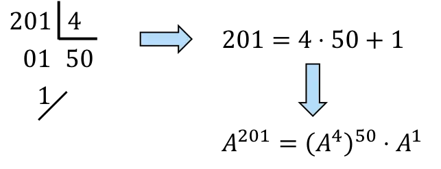
esercizio risolto passo passo delle potenze delle matrici 2x2 e della potenza n

$\displaystyle 201= 4 \cdot 50 +1$

,Ancora,

$A^{201}$

saranno 50 volte

$\displaystyle A^{4}$

e una volta

$\displaystyle A^{1}:$

$\displaystyle A^{201}=\left(A^4 \right)^{50} \cdot A^1$

E come lo sappiamo?

$\displaystyle A^4$

è la matrice identità

$\displaystyle I :$

$\displaystyle A^4 =I$

$\displaystyle A^{201}=\left(A^4 \right)^{50} \cdot A^1 = I^{50}\cdot A$

Inoltre, la matrice identità elevata a qualsiasi numero dà la matrice identità. Ancora:

$\displaystyle A^{201}= I^{50}\cdot A = I \cdot A$

E infine, qualsiasi matrice moltiplicata per la matrice identità dà la stessa matrice. COSÌ:

$\displaystyle A^{201}= I \cdot A = A$

Per quello

$A^{201}$

è uguale a

$A:$

$\displaystyle A^{201}= A =\begin{pmatrix} \bm{0} & \bm{-1} \\[1.1ex] \bm{1} & \bm{0} \end{pmatrix}$

Esercizio 5

Consideriamo la seguente matrice di ordine 3:

$\displaystyle A=\begin{pmatrix} 3 & 4 & -1 \\[1.1ex] -2 & -3 & 1 \\[1.1ex] -2 & -3 & 0 \end{pmatrix}$

Calcolare:

$\displaystyle A^{62}$

vedi soluzione

Ovviamente, calcola la potenza della matrice

$\displaystyle A^{62}$

Questo è un calcolo troppo grande per essere fatto a mano, quindi i poteri della matrice devono seguire uno schema. In questo caso è necessario calcolare

$\displaystyle A^{6}$

per conoscere la sequenza che seguono:

$\displaystyle A^2= A \cdot A = \begin{pmatrix}3 & 4 & -1 \\[1.1ex] -2 & -3 & 1 \\[1.1ex] -2 & -3 & 0 \end{pmatrix} \cdot \begin{pmatrix} 3 & 4 & -1 \\[1.1ex] -2 & -3 & 1 \\[1.1ex] -2 & -3 & 0 \end{pmatrix} = \begin{pmatrix} 3 & 3 & 1 \\[1.1ex] -2 & -2 & -1 \\[1.1ex] 0 & 1 & -1 \end{pmatrix}$

$\displaystyle A^3= A^2 \cdot A = \begin{pmatrix}3 & 3 & 1 \\[1.1ex] -2 & -2 & -1 \\[1.1ex] 0 & 1 & -1\end{pmatrix} \cdot \begin{pmatrix} 3 & 4 & -1 \\[1.1ex] -2 & -3 & 1 \\[1.1ex] -2 & -3 & 0 \end{pmatrix} = \begin{pmatrix} 1 & 0 & 0 \\[1.1ex] 0 & 1 & 0 \\[1.1ex] 0 & 0 & 1 \end{pmatrix}$

$\displaystyle A^4= A^3 \cdot A = \begin{pmatrix}1 & 0 & 0 \\[1.1ex] 0 & 1 & 0 \\[1.1ex] 0 & 0 & 1 \end{pmatrix} \cdot \begin{pmatrix} 3 & 4 & -1 \\[1.1ex] -2 & -3 & 1 \\[1.1ex] -2 & -3 & 0 \end{pmatrix} = \begin{pmatrix} 3 & 4 & -1 \\[1.1ex] -2 & -3 & 1 \\[1.1ex] -2 & -3 & 0 \end{pmatrix}$

$\displaystyle A^5= A^4 \cdot A = \begin{pmatrix}3 & 4 & -1 \\[1.1ex] -2 & -3 & 1 \\[1.1ex] -2 & -3 & 0 \end{pmatrix} \cdot \begin{pmatrix} 3 & 4 & -1 \\[1.1ex] -2 & -3 & 1 \\[1.1ex] -2 & -3 & 0 \end{pmatrix} = \begin{pmatrix} 3 & 3 & 1 \\[1.1ex] -2 & -2 & -1 \\[1.1ex] 0 & 1 & -1 \end{pmatrix}$

$\displaystyle A^6= A^5 \cdot A = \begin{pmatrix}3 & 3 & 1 \\[1.1ex] -2 & -2 & -1 \\[1.1ex] 0 & 1 & -1\end{pmatrix} \cdot \begin{pmatrix} 3 & 4 & -1 \\[1.1ex] -2 & -3 & 1 \\[1.1ex] -2 & -3 & 0 \end{pmatrix} = \begin{pmatrix} 1 & 0 & 0 \\[1.1ex] 0 & 1 & 0 \\[1.1ex] 0 & 0 & 1 \end{pmatrix}$

Con questi calcoli possiamo vedere che ogni 3 potenze otteniamo la matrice identità. Ci darà cioè come risultato la matrice identitaria dei poteri

$\displaystyle A^3$

$\displaystyle A^6$

$\displaystyle A^{9}$

$\displaystyle A^{12}$

,… In modo da calcolare

$\displaystyle A^{62}$

Dobbiamo scomporre 62 in multipli di 3:

esercizio risolto passo passo di una potenza di matrice 3x3, ennesima potenza

$\displaystyle 62= 3 \cdot 20 +2$

,Ancora,

$\displaystyle A^{62}$

saranno 20 volte

$\displaystyle A^{3}$

e una volta

$\displaystyle A^{2}:$

$\displaystyle A^{62}=\left(A^3 \right)^{20} \cdot A^2$

E come lo sappiamo?

$\displaystyle A^3$

è la matrice identità

$\displaystyle I :$

$\displaystyle A^3 =I$

$\displaystyle A^{62}=\left(A^3 \right)^{20} \cdot A^2 = I^{20}\cdot A^2$

Inoltre, la matrice identità elevata a qualsiasi numero dà la matrice identità. Ancora:

$\displaystyle A^{62}= I^{20}\cdot A^2 = I \cdot A^2$

Infine, qualsiasi matrice moltiplicata per la matrice identità dà la stessa matrice. Ancora:

$\displaystyle A^{62}= I \cdot A^2 = A^2$

Per quello

$A^{62}$

sarà uguale a

$A^{2}$

, per il quale abbiamo calcolato il risultato in precedenza:

$\displaystyle A^{62}= A^2=\begin{pmatrix} \bm{3} & \bm{3} & \bm{1} \\[1.1ex] \bm{-2} & \bm{-2} & \bm{-1} \\[1.1ex] \bm{0} & \bm{1} & \bm{-1} \end{pmatrix}$

Se questi esercizi sulle potenze delle matrici quadrate ti sono stati utili, puoi trovare risolti anche esercizi passo passo sull’addizione e sottrazione di matrici , una delle operazioni più utilizzate con le matrici.

Come si calcola la potenza di una matrice?

Esempio di calcolo della potenza di una matrice:

Qual è la potenza n di una matrice?

Esempio di calcolo della potenza n di una matrice:

Risolti i problemi di alimentazione della matrice

Esercizio 1

Esercizio 2

Esercizio 3

Esercizio 4

Esercizio 5

Lascia un commento Annulla risposta