Nesta página veremos como fazer potências de matrizes. Você também encontrará exemplos e exercícios resolvidos passo a passo de potências de matrizes que o ajudarão a entendê-lo perfeitamente. Você também aprenderá o que é a enésima potência de uma matriz e como encontrá-la.
Como é calculada a potência de uma matriz?
Para calcular a potência de uma matriz , você deve multiplicar a matriz por ela mesma quantas vezes o expoente indicar. Por exemplo:

Portanto, para obter a potência de uma matriz, você precisa saber como resolver a multiplicação de matrizes . Caso contrário, você não poderá calcular uma matriz de potência.
Exemplo de cálculo da potência de uma matriz:
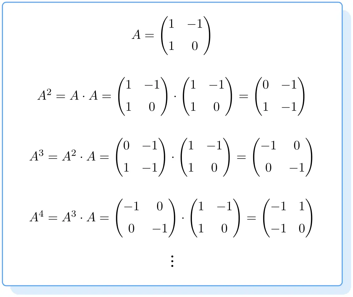
Portanto, a potência de uma matriz quadrada é calculada multiplicando a matriz por ela mesma. Da mesma forma, uma matriz cúbica é igual à matriz quadrada da própria matriz. Da mesma forma, para encontrar a potência de uma matriz elevada a quatro, a matriz elevada a três deve ser multiplicada pela própria matriz. E assim por diante.
Existe uma propriedade importante da potência da matriz que você deve conhecer: a potência de uma matriz só pode ser calculada quando ela é quadrada , ou seja, quando possui o mesmo número de linhas que de colunas.
Qual é a potência n de uma matriz?
A enésima potência de uma matriz é uma expressão que nos permite calcular facilmente qualquer potência de uma matriz.
Muitas vezes as potências das matrizes seguem um padrão . Portanto, se conseguirmos decifrar a sequência que seguem, poderemos calcular qualquer potência sem ter que fazer todas as multiplicações.
Isso significa que podemos encontrar uma fórmula que nos dê a enésima potência de uma matriz sem precisar calcular todas as potências.
Dicas para descobrir o padrão seguido pelos poderes:
- A paridade do expoente . Pode ser que poderes pares sejam de um lado e poderes ímpares de outro.
- Variação de sinais. Por exemplo, pode acontecer que os elementos de potências pares sejam positivos e os elementos de potências ímpares sejam negativos, ou vice-versa.
- Repetição: se a mesma matriz se repete a cada determinado número de potências ou não.
- Devemos também verificar se existe uma relação entre o expoente e os elementos da matriz.
Exemplo de cálculo da potência n de uma matriz:
- Ser

a seguinte matriz, calcule

E

.
![\displaystyle A = \begin{pmatrix} 1 & 1 \\[1.1ex] 1 & 1 \end{pmatrix}](https://mathority.org/wp-content/ql-cache/quicklatex.com-60016ce1c6799c93007526681fbf4894_l3.png "Rendered by QuickLaTeX.com")
Vamos primeiro calcular várias potências da matriz
, para tentar adivinhar o padrão seguido pelas potências. Então calculamos

,

,

E

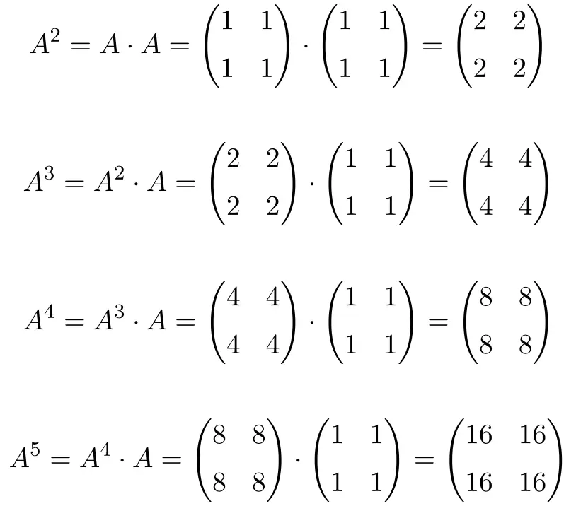
Ao calcular até

, vemos que as potências da matriz
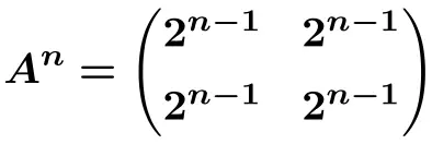
Elas seguem um padrão: para cada aumento de potência, o resultado é multiplicado por 2. Portanto, todas as matrizes são potências de 2:
![\displaystyle A^2= \begin{pmatrix} 2 & 2 \\[1.1ex] 2 & 2 \end{pmatrix} =\begin{pmatrix} 2^1 & 2^1 \\[1.1ex] 2^1 & 2^1 \end{pmatrix}](https://mathority.org/wp-content/ql-cache/quicklatex.com-4ec7ee835cf9eda6a4f9d497e8baff79_l3.png "Rendered by QuickLaTeX.com")
![\displaystyle A^3= \begin{pmatrix} 4 & 4 \\[1.1ex] 4 & 4 \end{pmatrix}=\begin{pmatrix} 2^2 & 2^2 \\[1.1ex] 2^2 & 2^2 \end{pmatrix}](https://mathority.org/wp-content/ql-cache/quicklatex.com-69c6ff0f4de92192584dadc4719167c7_l3.png "Rendered by QuickLaTeX.com")
![\displaystyle A^4= \begin{pmatrix} 8 & 8 \\[1.1ex] 8 & 8 \end{pmatrix}=\begin{pmatrix} 2^3 & 2^3 \\[1.1ex] 2^3 & 2^3 \end{pmatrix}](https://mathority.org/wp-content/ql-cache/quicklatex.com-f724a50b220b3026d53e40ee17870359_l3.png "Rendered by QuickLaTeX.com")
![\displaystyle A^5= \begin{pmatrix} 16 & 16 \\[1.1ex] 16 & 16 \end{pmatrix}=\begin{pmatrix} 2^4 & 2^4 \\[1.1ex] 2^4 & 2^4 \end{pmatrix}](https://mathority.org/wp-content/ql-cache/quicklatex.com-f5f08f7cc00465a6a098ce7d752aa66f_l3.png "Rendered by QuickLaTeX.com")
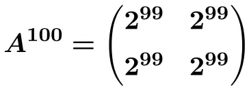
Podemos, portanto, derivar a fórmula para a enésima potência da matriz

E a partir desta fórmula podemos calcular

Problemas de potência de matriz resolvidos
Exercício 1
Considere a seguinte matriz de dimensão 2×2:
![\displaystyle A=\begin{pmatrix} 1 & 2 \\[1.1ex] -1 & 1 \end{pmatrix}](https://mathority.org/wp-content/ql-cache/quicklatex.com-cdf81cf9fb956a144c7bda96a84ec7db_l3.png "Rendered by QuickLaTeX.com")
Calcular:

Para calcular a potência de uma matriz, você deve multiplicar a matriz uma por uma. Portanto, primeiro calculamos

![\displaystyle A^2= A \cdot A = \begin{pmatrix} 1 & 2 \\[1.1ex] -1 & 1 \end{pmatrix} \cdot \begin{pmatrix} 1 & 2 \\[1.1ex] -1 & 1 \end{pmatrix} = \begin{pmatrix} -1 & 4 \\[1.1ex] -2 & -1\end{pmatrix}](https://mathority.org/wp-content/ql-cache/quicklatex.com-24916b0b0e4431b0a2ee2b09875dc903_l3.png "Rendered by QuickLaTeX.com")
Agora calculamos

![\displaystyle A^3= A^2 \cdot A = \begin{pmatrix} -1 & 4 \\[1.1ex] -2 & -1 \end{pmatrix} \cdot \begin{pmatrix} 1 & 2 \\[1.1ex] -1 & 1 \end{pmatrix} =\begin{pmatrix} -5 & 2 \\[1.1ex] -1 & -5 \end{pmatrix}](https://mathority.org/wp-content/ql-cache/quicklatex.com-57f79bd420c0044c84a64b431035b8ea_l3.png "Rendered by QuickLaTeX.com")
E finalmente calculamos

![\displaystyle A^4= A^3 \cdot A = \begin{pmatrix} -5 & 2 \\[1.1ex] -1 & -5 \end{pmatrix} \cdot \begin{pmatrix} 1 & 2 \\[1.1ex] -1 & 1 \end{pmatrix} = \begin{pmatrix} \bm{-7} & \bm{-8} \\[1.1ex] \bm{4} & \bm{-7} \end{pmatrix}](https://mathority.org/wp-content/ql-cache/quicklatex.com-bbc2ad8229ee141b323c9bbcc9df00fd_l3.png "Rendered by QuickLaTeX.com")
Exercício 2
Considere a seguinte matriz de ordem 2:
![\displaystyle A=\begin{pmatrix} 1 & 0 \\[1.1ex] 0 & 3 \end{pmatrix}](https://mathority.org/wp-content/ql-cache/quicklatex.com-33db03560b5c28f45eef9aa293484603_l3.png "Rendered by QuickLaTeX.com")
Calcular:

é uma potência muito grande para ser calculada manualmente, então as potências da matriz devem seguir um padrão. Então vamos calcular

para tentar entender a sequência que eles seguem:
![\displaystyle A^2= A \cdot A = \begin{pmatrix} 1 & 0 \\[1.1ex] 0 & 3 \end{pmatrix} \cdot \begin{pmatrix}1 & 0 \\[1.1ex] 0 & 3 \end{pmatrix} = \begin{pmatrix} 1 & 0 \\[1.1ex] 0 & 9 \end{pmatrix}](https://mathority.org/wp-content/ql-cache/quicklatex.com-cb9646cc984d754d2a618e6223e93cd3_l3.png "Rendered by QuickLaTeX.com")
![\displaystyle A^3= A^2 \cdot A = \begin{pmatrix} 1 & 0 \\[1.1ex] 0 & 9 \end{pmatrix} \cdot \begin{pmatrix}1 & 0 \\[1.1ex] 0 & 3 \end{pmatrix} = \begin{pmatrix} 1 & 0 \\[1.1ex] 0 & 27 \end{pmatrix}](https://mathority.org/wp-content/ql-cache/quicklatex.com-22fdee28399b9115de98a214ba0c8473_l3.png "Rendered by QuickLaTeX.com")
![\displaystyle A^4= A^3 \cdot A = \begin{pmatrix}1 & 0 \\[1.1ex] 0 & 27 \end{pmatrix} \cdot \begin{pmatrix}1 & 0 \\[1.1ex] 0 & 3 \end{pmatrix} = \begin{pmatrix} 1 & 0 \\[1.1ex] 0 & 81 \end{pmatrix}](https://mathority.org/wp-content/ql-cache/quicklatex.com-1a085a2338ce1e74885ca04bbd0011a7_l3.png "Rendered by QuickLaTeX.com")
![\displaystyle A^5= A^4 \cdot A = \begin{pmatrix}1 & 0 \\[1.1ex] 0 & 81 \end{pmatrix} \cdot \begin{pmatrix}1 & 0 \\[1.1ex] 0 & 3 \end{pmatrix} = \begin{pmatrix} 1 & 0 \\[1.1ex] 0 & 243 \end{pmatrix}](https://mathority.org/wp-content/ql-cache/quicklatex.com-3dc357146829da8323a0755fa16a8ca8_l3.png "Rendered by QuickLaTeX.com")
Desta forma podemos ver o padrão que as potências seguem: a cada potência, todos os números permanecem iguais, exceto o elemento da segunda coluna da segunda linha, que é multiplicado por 3. Portanto, todos os números permanecem sempre iguais. e o último elemento é uma potência de 3:
![\displaystyle A=\begin{pmatrix} 1 & 0 \\[1.1ex] 0 & 3 \end{pmatrix}=\begin{pmatrix} 1 & 0 \\[1.1ex] 0 & 3^1 \end{pmatrix}](https://mathority.org/wp-content/ql-cache/quicklatex.com-a0bfa34768808832e0fd5d3f730eb27b_l3.png "Rendered by QuickLaTeX.com")
![\displaystyle A^2=\begin{pmatrix} 1 & 0 \\[1.1ex] 0 & 9 \end{pmatrix}=\begin{pmatrix} 1 & 0 \\[1.1ex] 0 & 3^2 \end{pmatrix}](https://mathority.org/wp-content/ql-cache/quicklatex.com-f6e007f5ad5d38fd887d39f00bd2b9fc_l3.png "Rendered by QuickLaTeX.com")
![\displaystyle A^3=\begin{pmatrix} 1 & 0 \\[1.1ex] 0 & 27 \end{pmatrix}=\begin{pmatrix} 1 & 0 \\[1.1ex] 0 & 3^3 \end{pmatrix}](https://mathority.org/wp-content/ql-cache/quicklatex.com-585d8a00f418b50f60b4f95d87c5839c_l3.png "Rendered by QuickLaTeX.com")
![\displaystyle A^4=\begin{pmatrix} 1 & 0 \\[1.1ex] 0 & 81 \end{pmatrix}=\begin{pmatrix} 1 & 0 \\[1.1ex] 0 & 3^4 \end{pmatrix}](https://mathority.org/wp-content/ql-cache/quicklatex.com-dec6b9db4b59d9759adf85cee442cca3_l3.png "Rendered by QuickLaTeX.com")
![\displaystyle A^5=\begin{pmatrix} 1 & 0 \\[1.1ex] 0 & 243 \end{pmatrix}=\begin{pmatrix} 1 & 0 \\[1.1ex] 0 & 3^5 \end{pmatrix}](https://mathority.org/wp-content/ql-cache/quicklatex.com-f7244b46950df4d9107cbdb7ad004e17_l3.png "Rendered by QuickLaTeX.com")
Portanto, a fórmula para a enésima potência da matriz

Leste:
![\displaystyle A^n=\begin{pmatrix} 1 & 0 \\[1.1ex] 0 & 3^n\end{pmatrix}](https://mathority.org/wp-content/ql-cache/quicklatex.com-beec2f1ed3e47902de0f25fe1901e294_l3.png "Rendered by QuickLaTeX.com")
E a partir desta fórmula podemos calcular

![\displaystyle\bm{A^{35}=}\begin{pmatrix} \bm{1} & \bm{0} \\[1.1ex] \bm{0} & \bm{3^{35}}\end{pmatrix}](https://mathority.org/wp-content/ql-cache/quicklatex.com-aa3261646ca7bfa41f8ad46331a0af4b_l3.png "Rendered by QuickLaTeX.com")
Exercício 3
Considere a seguinte matriz 3×3:
![\displaystyle A=\begin{pmatrix} 1 & \frac{1}{5} & \frac{1}{5} \\[1.1ex] 0 & 1 & 0 \\[1.1ex] 0 & 0 & 1 \end{pmatrix}](https://mathority.org/wp-content/ql-cache/quicklatex.com-f11fe8a7dcd1e308faa0af24eee3f362_l3.png "Rendered by QuickLaTeX.com")
Calcular:

é uma potência muito grande para ser calculada manualmente, então as potências da matriz devem seguir um padrão. Então vamos calcular
para tentar entender a sequência que eles seguem:
![\displaystyle A^2= A \cdot A = \begin{pmatrix} 1 & \frac{1}{5} & \frac{1}{5} \\[1.1ex] 0 & 1 & 0 \\[1.1ex] 0 & 0 & 1 \end{pmatrix} \cdot \begin{pmatrix}1 & \frac{1}{5} & \frac{1}{5} \\[1.1ex] 0 & 1 & 0 \\[1.1ex] 0 & 0 & 1 \end{pmatrix} = \begin{pmatrix} 1 & \frac{2}{5} & \frac{2}{5} \\[1.1ex] 0 & 1 & 0 \\[1.1ex] 0 & 0 & 1 \end{pmatrix}](https://mathority.org/wp-content/ql-cache/quicklatex.com-acb15d7f461d11e3668bc0b96a1fdc06_l3.png "Rendered by QuickLaTeX.com")
![\displaystyle A^3= A^2 \cdot A = \begin{pmatrix} 1 & \frac{2}{5} & \frac{2}{5} \\[1.1ex] 0 & 1 & 0 \\[1.1ex] 0 & 0 & 1\end{pmatrix} \cdot \begin{pmatrix}1 & \frac{1}{5} & \frac{1}{5} \\[1.1ex] 0 & 1 & 0 \\[1.1ex] 0 & 0 & 1 \end{pmatrix} = \begin{pmatrix} 1 & \frac{3}{5} & \frac{3}{5} \\[1.1ex] 0 & 1 & 0 \\[1.1ex] 0 & 0 & 1 \end{pmatrix}](https://mathority.org/wp-content/ql-cache/quicklatex.com-f416625ded948830fa80799249c12608_l3.png "Rendered by QuickLaTeX.com")
![\displaystyle A^4= A^3 \cdot A = \begin{pmatrix} 1 & \frac{3}{5} & \frac{3}{5} \\[1.1ex] 0 & 1 & 0 \\[1.1ex] 0 & 0 & 1\end{pmatrix} \cdot \begin{pmatrix}1 & \frac{1}{5} & \frac{1}{5} \\[1.1ex] 0 & 1 & 0 \\[1.1ex] 0 & 0 & 1 \end{pmatrix} = \begin{pmatrix} 1 & \frac{4}{5} & \frac{4}{5} \\[1.1ex] 0 & 1 & 0 \\[1.1ex] 0 & 0 & 1 \end{pmatrix}](https://mathority.org/wp-content/ql-cache/quicklatex.com-a76fd60051b157f06c2a731ff575d1e5_l3.png "Rendered by QuickLaTeX.com")
![\displaystyle A^5= A^4 \cdot A = \begin{pmatrix} 1 & \frac{4}{5} & \frac{4}{5} \\[1.1ex] 0 & 1 & 0 \\[1.1ex] 0 & 0 & 1\end{pmatrix} \cdot \begin{pmatrix}1 & \frac{1}{5} & \frac{1}{5} \\[1.1ex] 0 & 1 & 0 \\[1.1ex] 0 & 0 & 1 \end{pmatrix} = \begin{pmatrix} 1 & \frac{5}{5} & \frac{5}{5} \\[1.1ex] 0 & 1 & 0 \\[1.1ex] 0 & 0 & 1 \end{pmatrix}](https://mathority.org/wp-content/ql-cache/quicklatex.com-3409c7b8d82ffd21cc084a12405fce74_l3.png "Rendered by QuickLaTeX.com")
Desta forma podemos ver o padrão que as potências seguem: a cada potência, todos os números permanecem iguais, exceto as frações, que aumentam uma unidade no numerador:
![\displaystyle A=\begin{pmatrix} 1 & \frac{1}{5} & \frac{1}{5} \\[1.1ex] 0 & 1 & 0 \\[1.1ex] 0 & 0 & 1 \end{pmatrix}](https://mathority.org/wp-content/ql-cache/quicklatex.com-86c72aa2b21e7a68bbebfe7af5daa420_l3.png "Rendered by QuickLaTeX.com")
![\displaystyle A^2= \begin{pmatrix} 1 & \frac{2}{5} & \frac{2}{5} \\[1.1ex] 0 & 1 & 0 \\[1.1ex] 0 & 0 & 1 \end{pmatrix}](https://mathority.org/wp-content/ql-cache/quicklatex.com-ce805455e49bf018f8f22588391ac44c_l3.png "Rendered by QuickLaTeX.com")
![\displaystyle A^3= \begin{pmatrix} 1 & \frac{3}{5} & \frac{3}{5} \\[1.1ex] 0 & 1 & 0 \\[1.1ex] 0 & 0 & 1 \end{pmatrix}](https://mathority.org/wp-content/ql-cache/quicklatex.com-bd5468ece9001274493687f3786b0af3_l3.png "Rendered by QuickLaTeX.com")
![\displaystyle A^4= \begin{pmatrix} 1 & \frac{4}{5} & \frac{4}{5} \\[1.1ex] 0 & 1 & 0 \\[1.1ex] 0 & 0 & 1 \end{pmatrix}](https://mathority.org/wp-content/ql-cache/quicklatex.com-07fd0e03c0163b58fffbe0235009fd8e_l3.png "Rendered by QuickLaTeX.com")
![\displaystyle A^5= \begin{pmatrix} 1 & \frac{5}{5} & \frac{5}{5} \\[1.1ex] 0 & 1 & 0 \\[1.1ex] 0 & 0 & 1 \end{pmatrix}](https://mathority.org/wp-content/ql-cache/quicklatex.com-5ea88723757d1f2d8d6de1ac2d3843c7_l3.png "Rendered by QuickLaTeX.com")
Portanto, a fórmula para a potência da enésima matriz
Leste:
![\displaystyle A^n= \begin{pmatrix} 1 & \frac{n}{5} & \frac{n}{5} \\[1.1ex] 0 & 1 & 0 \\[1.1ex] 0 & 0 & 1 \end{pmatrix}](https://mathority.org/wp-content/ql-cache/quicklatex.com-56308ff348d67ba1aba5816d85e9ee1c_l3.png "Rendered by QuickLaTeX.com")
E a partir desta fórmula podemos calcular

![\displaystyle A^{100}= \begin{pmatrix} 1 & \frac{100}{5} & \frac{100}{5} \\[1.1ex] 0 & 1 & 0 \\[1.1ex] 0 & 0 & 1 \end{pmatrix}= \begin{pmatrix} \bm{1} & \bm{20} & \bm{20} \\[1.1ex] \bm{0} & \bm{1} & \bm{0} \\[1.1ex] \bm{0} & \bm{0} & \bm{1} \end{pmatrix}](https://mathority.org/wp-content/ql-cache/quicklatex.com-5352f021f5ab30e999c57f978ff55ad6_l3.png "Rendered by QuickLaTeX.com")
Exercício 4
Considere a seguinte matriz de tamanho 2×2:
![\displaystyle A=\begin{pmatrix} 0 & -1 \\[1.1ex] 1 & 0 \end{pmatrix}](https://mathority.org/wp-content/ql-cache/quicklatex.com-4609248b534d656aa9495b58f42e343f_l3.png "Rendered by QuickLaTeX.com")
Calcular:

é uma potência muito grande para ser calculada manualmente, então as potências da matriz devem seguir um padrão. Neste caso é necessário calcular

para saber a sequência que seguem:
![\displaystyle A^2= A \cdot A = \begin{pmatrix} 0 & -1 \\[1.1ex] 1 & 0 \end{pmatrix} \cdot \begin{pmatrix} 0 & -1 \\[1.1ex] 1 & 0 \end{pmatrix} = \begin{pmatrix} -1 & 0 \\[1.1ex] 0 & -1 \end{pmatrix}](https://mathority.org/wp-content/ql-cache/quicklatex.com-c9a1fb4cf8bb75cf02d76a26054e6bfa_l3.png "Rendered by QuickLaTeX.com")
![\displaystyle A^3= A^2 \cdot A = \begin{pmatrix} -1 & 0 \\[1.1ex] 0 & -1 \end{pmatrix} \cdot \begin{pmatrix} 0 & -1 \\[1.1ex] 1 & 0 \end{pmatrix} = \begin{pmatrix} 0 & 1 \\[1.1ex] -1 & 0 \end{pmatrix}](https://mathority.org/wp-content/ql-cache/quicklatex.com-110c4b30c78811cafdd4234e128ed414_l3.png "Rendered by QuickLaTeX.com")
![\displaystyle A^4= A^3 \cdot A = \begin{pmatrix}0 & 1 \\[1.1ex] -1 & 0 \end{pmatrix} \cdot \begin{pmatrix} 0 & -1 \\[1.1ex] 1 & 0 \end{pmatrix} = \begin{pmatrix} 1 & 0 \\[1.1ex] 0 & 1 \end{pmatrix} = \bm{I}](https://mathority.org/wp-content/ql-cache/quicklatex.com-2b1976bbdf3c1daa9d75497efc07975c_l3.png "Rendered by QuickLaTeX.com")
![\displaystyle A^5= A^4 \cdot A = \begin{pmatrix} 1 & 0 \\[1.1ex] 0 & 1\end{pmatrix} \cdot \begin{pmatrix} 0 & -1 \\[1.1ex] 1 & 0 \end{pmatrix} = \begin{pmatrix} 0 & -1 \\[1.1ex] 1 & 0 \end{pmatrix}](https://mathority.org/wp-content/ql-cache/quicklatex.com-e0266d832a2fc0a04c9f6582dc231d57_l3.png "Rendered by QuickLaTeX.com")
![\displaystyle A^6= A^5 \cdot A = \begin{pmatrix} 0 & -1 \\[1.1ex] 1 & 0 \end{pmatrix} \cdot \begin{pmatrix} 0 & -1 \\[1.1ex] 1 & 0 \end{pmatrix} = \begin{pmatrix} -1 & 0 \\[1.1ex] 0 & -1 \end{pmatrix}](https://mathority.org/wp-content/ql-cache/quicklatex.com-21dea9844b7bfdb990bbb2bc955c866e_l3.png "Rendered by QuickLaTeX.com")
![\displaystyle A^7= A^6 \cdot A = \begin{pmatrix} -1 & 0 \\[1.1ex] 0 & -1 \end{pmatrix} \cdot \begin{pmatrix} 0 & -1 \\[1.1ex] 1 & 0 \end{pmatrix} = \begin{pmatrix} 0 & 1 \\[1.1ex] -1 & 0 \end{pmatrix}](https://mathority.org/wp-content/ql-cache/quicklatex.com-788e75a71c1dfe4a60f0e52960715efe_l3.png "Rendered by QuickLaTeX.com")
![\displaystyle A^8= A^7 \cdot A = \begin{pmatrix}0 & 1 \\[1.1ex] -1 & 0 \end{pmatrix} \cdot \begin{pmatrix} 0 & -1 \\[1.1ex] 1 & 0 \end{pmatrix} = \begin{pmatrix} 1 & 0 \\[1.1ex] 0 & 1 \end{pmatrix} = \bm{I}](https://mathority.org/wp-content/ql-cache/quicklatex.com-4947286a163847383e3735a508b0037d_l3.png "Rendered by QuickLaTeX.com")
Com esses cálculos podemos ver que a cada 4 potências obtemos a matriz identidade. Isso quer dizer que nos dará como resultado a matriz identidade dos poderes
,

,

,

,… Então, para calcular
devemos decompor 201 em múltiplos de 4:
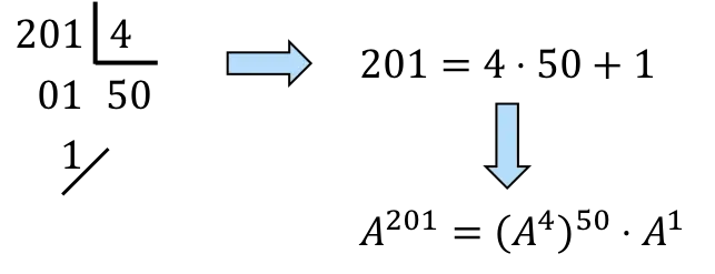

,Ainda,

serão 50 vezes

e uma vez


E como sabemos disso
é a matriz identidade


Além disso, a matriz identidade elevada a qualquer número fornece a matriz identidade. Ainda:

E, finalmente, qualquer matriz multiplicada pela matriz identidade dá a mesma matriz. ENTÃO:

Para que
é igual a
![\displaystyle A^{201}= A =\begin{pmatrix} \bm{0} & \bm{-1} \\[1.1ex] \bm{1} & \bm{0} \end{pmatrix}](https://mathority.org/wp-content/ql-cache/quicklatex.com-1214abe876a5aede8fbbce79009d5dbc_l3.png "Rendered by QuickLaTeX.com")
Exercício 5
Considere a seguinte matriz de ordem 3:
![\displaystyle A=\begin{pmatrix} 3 & 4 & -1 \\[1.1ex] -2 & -3 & 1 \\[1.1ex] -2 & -3 & 0 \end{pmatrix}](https://mathority.org/wp-content/ql-cache/quicklatex.com-b8f3ba8b2d15b622f99774be05aa2620_l3.png "Rendered by QuickLaTeX.com")
Calcular:

Obviamente, calcule a potência da matriz
Este é um cálculo muito grande para ser feito manualmente, então as potências da matriz devem seguir um padrão. Neste caso é necessário calcular

para saber a sequência que seguem:
![\displaystyle A^2= A \cdot A = \begin{pmatrix}3 & 4 & -1 \\[1.1ex] -2 & -3 & 1 \\[1.1ex] -2 & -3 & 0 \end{pmatrix} \cdot \begin{pmatrix} 3 & 4 & -1 \\[1.1ex] -2 & -3 & 1 \\[1.1ex] -2 & -3 & 0 \end{pmatrix} = \begin{pmatrix} 3 & 3 & 1 \\[1.1ex] -2 & -2 & -1 \\[1.1ex] 0 & 1 & -1 \end{pmatrix}](https://mathority.org/wp-content/ql-cache/quicklatex.com-4032b55d68a5615911a5b7c997b05e6f_l3.png "Rendered by QuickLaTeX.com")
![\displaystyle A^3= A^2 \cdot A = \begin{pmatrix}3 & 3 & 1 \\[1.1ex] -2 & -2 & -1 \\[1.1ex] 0 & 1 & -1\end{pmatrix} \cdot \begin{pmatrix} 3 & 4 & -1 \\[1.1ex] -2 & -3 & 1 \\[1.1ex] -2 & -3 & 0 \end{pmatrix} = \begin{pmatrix} 1 & 0 & 0 \\[1.1ex] 0 & 1 & 0 \\[1.1ex] 0 & 0 & 1 \end{pmatrix}](https://mathority.org/wp-content/ql-cache/quicklatex.com-8b5deef2a7728c5e82e1a1dafb1a939c_l3.png "Rendered by QuickLaTeX.com")
![\displaystyle A^4= A^3 \cdot A = \begin{pmatrix}1 & 0 & 0 \\[1.1ex] 0 & 1 & 0 \\[1.1ex] 0 & 0 & 1 \end{pmatrix} \cdot \begin{pmatrix} 3 & 4 & -1 \\[1.1ex] -2 & -3 & 1 \\[1.1ex] -2 & -3 & 0 \end{pmatrix} = \begin{pmatrix} 3 & 4 & -1 \\[1.1ex] -2 & -3 & 1 \\[1.1ex] -2 & -3 & 0 \end{pmatrix}](https://mathority.org/wp-content/ql-cache/quicklatex.com-f62e856d037138b2ead39b17ccebf96d_l3.png "Rendered by QuickLaTeX.com")
![\displaystyle A^5= A^4 \cdot A = \begin{pmatrix}3 & 4 & -1 \\[1.1ex] -2 & -3 & 1 \\[1.1ex] -2 & -3 & 0 \end{pmatrix} \cdot \begin{pmatrix} 3 & 4 & -1 \\[1.1ex] -2 & -3 & 1 \\[1.1ex] -2 & -3 & 0 \end{pmatrix} = \begin{pmatrix} 3 & 3 & 1 \\[1.1ex] -2 & -2 & -1 \\[1.1ex] 0 & 1 & -1 \end{pmatrix}](https://mathority.org/wp-content/ql-cache/quicklatex.com-854da5c09b6662da46acb790afb6d01a_l3.png "Rendered by QuickLaTeX.com")
![\displaystyle A^6= A^5 \cdot A = \begin{pmatrix}3 & 3 & 1 \\[1.1ex] -2 & -2 & -1 \\[1.1ex] 0 & 1 & -1\end{pmatrix} \cdot \begin{pmatrix} 3 & 4 & -1 \\[1.1ex] -2 & -3 & 1 \\[1.1ex] -2 & -3 & 0 \end{pmatrix} = \begin{pmatrix} 1 & 0 & 0 \\[1.1ex] 0 & 1 & 0 \\[1.1ex] 0 & 0 & 1 \end{pmatrix}](https://mathority.org/wp-content/ql-cache/quicklatex.com-c9f804a1c129e18d105fb92254c971fa_l3.png "Rendered by QuickLaTeX.com")
Com esses cálculos podemos ver que a cada 3 potências obtemos a matriz identidade. Isso quer dizer que nos dará como resultado a matriz identidade dos poderes

,

,

,
,… Então isso para calcular
Devemos decompor 62 em múltiplos de 3:


,Ainda,
serão 20 vezes

e uma vez


E como sabemos disso
é a matriz identidade


Além disso, a matriz identidade elevada a qualquer número fornece a matriz identidade. Ainda:

Finalmente, qualquer matriz multiplicada pela matriz identidade dá a mesma matriz. Ainda:

Para que

será igual a

, para o qual calculamos o resultado anteriormente:
![\displaystyle A^{62}= A^2=\begin{pmatrix} \bm{3} & \bm{3} & \bm{1} \\[1.1ex] \bm{-2} & \bm{-2} & \bm{-1} \\[1.1ex] \bm{0} & \bm{1} & \bm{-1} \end{pmatrix}](https://mathority.org/wp-content/ql-cache/quicklatex.com-3f95e17aacde501ca1c28dbf14324f0b_l3.png "Rendered by QuickLaTeX.com")
Se esses exercícios sobre potências de matrizes quadradas foram úteis para você, você também pode encontrar exercícios passo a passo resolvidos sobre adição e subtração de matrizes , uma das operações com matrizes mais utilizadas.