Nesta página você aprenderá o que é e como calcular a inversa de uma matriz pelo método dos determinantes (ou matriz adjunta) e pelo método de Gauss. Você também verá todas as propriedades da matriz inversa e também encontrará exemplos e exercícios resolvidos passo a passo para cada método, para que você os compreenda completamente. Por fim, explicamos uma fórmula para inverter rapidamente uma matriz 2×2 e ainda a maior utilidade desta operação matricial: resolver um sistema de equações lineares.
Qual é o inverso de uma matriz?
Ser

uma matriz quadrada. A matriz inversa de
Esta escrevendo

, e é esta matriz que satisfaz:


Ouro

é a matriz de identidade.
Quando você pode inverter uma matriz e quando não?
A maneira mais simples de determinar a invertibilidade de uma matriz é usar seu determinante:
- Se o determinante da matriz em questão for diferente de 0, isso significa que a matriz é invertível. Neste caso dizemos que é uma matriz regular. Além disso, isso implica que a matriz tem classificação máxima.
- Por outro lado, se o determinante da matriz for igual a 0, a matriz não pode ser invertida. E, neste caso, dizemos que se trata de uma matriz singular ou degenerada.
Principalmente, existem dois métodos para inverter qualquer matriz: o método dos determinantes ou matriz adjunta e o método de Gauss. Abaixo você tem a explicação do primeiro, mas também pode consultar abaixo como inverter uma matriz com o método Gauss.
Inverta uma matriz usando o método do determinante (ou usando a matriz adjacente)
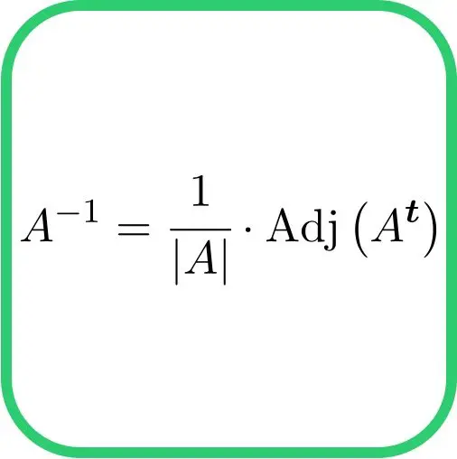
Para calcular o inverso de uma matriz ,

, a seguinte fórmula deve ser aplicada:

Ouro:
-

é o determinante da matriz
-

é a matriz adjunta de
- O expositor

indica transposição de matriz, ou seja, a matriz anexada deve ser transposta.
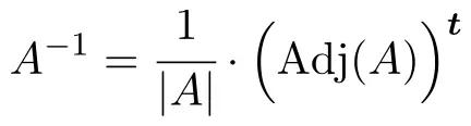
Comentário: Alguns livros usam uma fórmula de matriz inversa ligeiramente diferente: eles primeiro transpõem a matriz A e depois calculam sua matriz adjunta, em vez de primeiro calcular a matriz adjunta e depois transpô-la. Na realidade, a ordem não importa porque o resultado é exatamente o mesmo. Deixamos aqui a fórmula para inverter uma matriz modificada caso você prefira usar esta:
Veremos então como encontrar o inverso de uma matriz resolvendo um exercício como exemplo:
Exemplo de cálculo da matriz inversa usando o método determinante (ou matriz adjunta):
- Calcule o inverso da seguinte matriz:
![\displaystyle A = \begin{pmatrix} 4 & -2 \\[1.1ex] 3 & -1 \end{pmatrix}](https://mathority.org/wp-content/ql-cache/quicklatex.com-c37ec4a7afd5b313bcf3c50d6ce26c6d_l3.png "Rendered by QuickLaTeX.com")
Para determinar o inverso da matriz, devemos aplicar a seguinte fórmula:
Mas se o determinante da matriz for zero isso significa que a matriz não é invertível. Portanto, a primeira coisa a fazer é calcular o determinante da matriz e verificar se ele é diferente de 0:
![\displaystyle \lvert A \rvert = \begin{vmatrix} 4 & -2 \\[1.1ex] 3 & -1 \end{vmatrix} = -4- (-6) = 2](https://mathority.org/wp-content/ql-cache/quicklatex.com-710ccd4e4912dd492b496a742eaf7f56_l3.png "Rendered by QuickLaTeX.com")
O determinante não é 0 , então a matriz é invertível .
Portanto, substituindo o valor do determinante na fórmula, o inverso da matriz será:

Devemos agora calcular a matriz suplente de A. Para fazer isso, devemos substituir cada elemento da matriz A pelo seu substituto.
Lembre-se que para calcular o anexo de

, isto é, do elemento linha

e a coluna

, a seguinte fórmula deve ser aplicada:

Onde o complementar menor de
é o determinante da matriz eliminando a linha
e a coluna
.
Assim, os deputados dos elementos da matriz A são:


Comentário: Não confunda o determinante 1×1 com o valor absoluto, pois no determinante 1×1 o número não é convertido em positivo.
Uma vez calculados os deputados, basta substituir os elementos de A pelos seus deputados para encontrar a matriz de deputados de A :
![\displaystyle \displaystyle \text{Adj}(A) = \begin{pmatrix} -1 & -3 \\[1.1ex] 2 & 4 \end{pmatrix}](https://mathority.org/wp-content/ql-cache/quicklatex.com-08fb7666b4518399c2a469ba445762be_l3.png "Rendered by QuickLaTeX.com")
Comentário: em certos locais a matriz adjunta é a transposta da matriz adjunta que definimos aqui.
Portanto, substituímos a matriz anexa na fórmula da matriz inversa e ela se torna:
![\displaystyle A^{-1} = \cfrac{1}{2} \cdot \begin{pmatrix} -1 & -3 \\[1.1ex] 2 & 4 \end{pmatrix} ^{\bm{t}}](https://mathority.org/wp-content/ql-cache/quicklatex.com-0abb4127db9c3c1d0a7b669fbc782605_l3.png "Rendered by QuickLaTeX.com")
O expositor
Isso nos diz que precisamos transpor a matriz . E para transpor uma matriz é preciso transformar suas linhas em colunas , ou seja, a primeira linha da matriz passa a ser a primeira coluna da matriz, e a segunda linha passa a ser a segunda coluna:
![\displaystyle A^{-1} = \cfrac{1}{2} \cdot \begin{pmatrix} -1 & 2 \\[1.1ex] -3 & 4 \end{pmatrix}](https://mathority.org/wp-content/ql-cache/quicklatex.com-22965912cf8aee99610c81cf575c0ecd_l3.png "Rendered by QuickLaTeX.com")
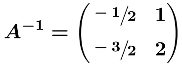
E finalmente, multiplicamos cada termo da matriz por

![\displaystyle A^{-1} = \begin{pmatrix} \sfrac{-1}{2} & \sfrac{2}{2} \\[1.1ex] \sfrac{-3}{2} & \sfrac{4}{2} \end{pmatrix}](https://mathority.org/wp-content/ql-cache/quicklatex.com-220748840151b429919c7ce6587b1bc0_l3.png "Rendered by QuickLaTeX.com")
Exercícios resolvidos sobre matrizes inversas com o método dos determinantes (ou a matriz adjacente)
Exercício 1
Inverta a seguinte matriz de dimensão 2×2 usando o método da matriz adjunta:
![\displaystyle A=\begin{pmatrix} 1 & 3 \\[1.1ex] 2 & 7 \end{pmatrix}](https://mathority.org/wp-content/ql-cache/quicklatex.com-bfb0807249e78845b375a402eb23a32b_l3.png "Rendered by QuickLaTeX.com")
A fórmula da matriz inversa é:
Primeiro calculamos o determinante da matriz:
![\displaystyle \begin{vmatrix}A\end{vmatrix}=\begin{vmatrix} 1 & 3 \\[1.1ex] 2 & 7 \end{vmatrix} = 7-6 = 1](https://mathority.org/wp-content/ql-cache/quicklatex.com-1c4e3bac90eb0da0361b4be1a2225146_l3.png "Rendered by QuickLaTeX.com")
O determinante é diferente de 0, então a matriz pode ser invertida.
Vamos agora calcular a matriz adjunta de A:


![\displaystyle \displaystyle \text{Adj}(A) = \begin{pmatrix} 7 & -2 \\[1.1ex] -3 & 1 \end{pmatrix}](https://mathority.org/wp-content/ql-cache/quicklatex.com-3dea8fca2c025ff9b7d7673904344996_l3.png "Rendered by QuickLaTeX.com")
Uma vez calculado o determinante da matriz e seu adjunto, substituímos seus valores na fórmula:
![\displaystyle A^{-1} = \cfrac{1}{1} \cdot \begin{pmatrix} 7 & -2 \\[1.1ex] -3 & 1 \end{pmatrix}^{\bm{t}}](https://mathority.org/wp-content/ql-cache/quicklatex.com-9475e4162eff7e1ed9c08f363a8279ec_l3.png "Rendered by QuickLaTeX.com")
Transpomos a matriz anexa:
![\displaystyle A^{-1} = 1 \cdot \begin{pmatrix} 7 & -3 \\[1.1ex] -2 & 1 \end{pmatrix}](https://mathority.org/wp-content/ql-cache/quicklatex.com-a5a6aaa8168e55c6eab1e3be1229a3da_l3.png "Rendered by QuickLaTeX.com")
A matriz inversa de A é portanto:
![\displaystyle \bm{A^{-1} =} \begin{pmatrix} \bm{7} & \bm{-3} \\[1.1ex] \bm{-2} & \bm{1} \end{pmatrix}](https://mathority.org/wp-content/ql-cache/quicklatex.com-1236ad7262705dbbd9b0a094084ceac5_l3.png "Rendered by QuickLaTeX.com")
Exercício 2
Inverta a seguinte matriz quadrada usando o método do determinante:
![\displaystyle A=\begin{pmatrix} -3 & -2 \\[1.1ex] 5 & 4 \end{pmatrix}](https://mathority.org/wp-content/ql-cache/quicklatex.com-eb735917d200ed35918cd44be6bd155b_l3.png "Rendered by QuickLaTeX.com")
A fórmula da matriz inversa é:
Primeiro calculamos o determinante da matriz:
![\displaystyle \begin{vmatrix}A\end{vmatrix}=\begin{vmatrix} -3 & -2 \\[1.1ex] 5 & 4\end{vmatrix} = -12+10 = -2](https://mathority.org/wp-content/ql-cache/quicklatex.com-49cd3daf7c50c811e78c29efe036bda4_l3.png "Rendered by QuickLaTeX.com")
O determinante é diferente de 0, então a matriz pode ser invertida.
Vamos agora calcular a matriz adjunta de A:


![\displaystyle \displaystyle \text{Adj}(A) = \begin{pmatrix} 4 & -5 \\[1.1ex] 2 & -3 \end{pmatrix}](https://mathority.org/wp-content/ql-cache/quicklatex.com-208ab7161076485ca6928bd1208f6714_l3.png "Rendered by QuickLaTeX.com")
Uma vez encontrado o determinante da matriz e seu adjunto, substituímos seus valores na fórmula:
![\displaystyle A^{-1} = \cfrac{1}{-2} \cdot \begin{pmatrix} 4 & -5 \\[1.1ex] 2 & -3 \end{pmatrix}^{\bm{t}}](https://mathority.org/wp-content/ql-cache/quicklatex.com-babecc87455bdc54006a77ba5369e540_l3.png "Rendered by QuickLaTeX.com")
Transpomos a matriz anexa:
![\displaystyle A^{-1} = \cfrac{1}{-2} \cdot \begin{pmatrix} 4 & 2 \\[1.1ex] -5 & -3 \end{pmatrix}](https://mathority.org/wp-content/ql-cache/quicklatex.com-17529597656a112a27d136ca212834d8_l3.png "Rendered by QuickLaTeX.com")
Multiplicamos cada elemento por

![\displaystyle A^{-1} = \begin{pmatrix} \cfrac{4}{-2} & \cfrac{2}{-2} \\[3ex] \cfrac{-5}{-2} & \cfrac{-3}{-2} \end{pmatrix}](https://mathority.org/wp-content/ql-cache/quicklatex.com-be52d2df839244cbb0b0ee00c9e45265_l3.png "Rendered by QuickLaTeX.com")
A matriz inversa de A é portanto:
![\displaystyle \bm{A^{-1} =} \begin{pmatrix} \bm{-2} & \bm{-1} \\[2ex] \cfrac{\bm{5}}{\bm{2}} & \cfrac{\bm{3}}{\bm{2}} \end{pmatrix}](https://mathority.org/wp-content/ql-cache/quicklatex.com-13e218c7d075daba3f875345f324d001_l3.png "Rendered by QuickLaTeX.com")
Exercício 3
Inverta a seguinte matriz de dimensão 3×3 usando o método da matriz adjunta:
![\displaystyle A=\begin{pmatrix}2&3&-2\\[1.1ex] 1&4&1\\[1.1ex] 2&1&-3\end{pmatrix}](https://mathority.org/wp-content/ql-cache/quicklatex.com-d1b6a5f638281754d80983b5a50e15be_l3.png "Rendered by QuickLaTeX.com")
A fórmula da matriz inversa é:
Primeiro resolvemos o determinante da matriz com a regra de Sarrus:
![\displaystyle \begin{vmatrix}A\end{vmatrix}=\begin{vmatrix} 2&3&-2\\[1.1ex] 1&4&1\\[1.1ex] 2&1&-3 \end{vmatrix} = -24+6-2+16-2+9 = 3](https://mathority.org/wp-content/ql-cache/quicklatex.com-fcac1cb3935b1000b6493a2866e8728a_l3.png "Rendered by QuickLaTeX.com")
O determinante é diferente de 0, então a matriz pode ser invertida.
Uma vez resolvido o determinante, encontramos a matriz adjunta de A:
![\text{Adjunto de 2} = \displaystyle (-1)^{1+1} \bm{\cdot} \begin{vmatrix} 4&1\\[1.1ex] 1&-3 \end{vmatrix} = 1 \cdot (-13) = \bm{-13}](https://mathority.org/wp-content/ql-cache/quicklatex.com-c510482ac77a8c5d511c095de600f1ba_l3.png "Rendered by QuickLaTeX.com")
![\text{Adjunto de 3} = \displaystyle (-1)^{1+2} \bm{\cdot} \begin{vmatrix}1&1\\[1.1ex] 2&-3\end{vmatrix} = -1 \cdot (-5) = \bm{5}](https://mathority.org/wp-content/ql-cache/quicklatex.com-fa99e03d34c925098c1ad3ed6f06c745_l3.png "Rendered by QuickLaTeX.com")
![\text{Adjunto de -2} = \displaystyle (-1)^{1+3} \bm{\cdot} \begin{vmatrix} 1&4\\[1.1ex] 2&1 \end{vmatrix} = 1\cdot (-7) = \bm{-7}](https://mathority.org/wp-content/ql-cache/quicklatex.com-3bf9f8565b3e4a99ff254c7558699c13_l3.png "Rendered by QuickLaTeX.com")
![\text{Adjunto de 1} = \displaystyle (-1)^{2+1} \bm{\cdot} \begin{vmatrix} 3&-2 \\[1.1ex] 1&-3 \end{vmatrix} = -1 \cdot (-7) = \bm{7}](https://mathority.org/wp-content/ql-cache/quicklatex.com-99e2c3f55fbba7b5faa014758b60f4a8_l3.png "Rendered by QuickLaTeX.com")
![\text{Adjunto de 4} = \displaystyle (-1)^{2+2} \bm{\cdot} \begin{vmatrix} 2&-2\\[1.1ex] 2&-3 \end{vmatrix} = 1 \cdot (-2) = \bm{-2}](https://mathority.org/wp-content/ql-cache/quicklatex.com-23326bccecf752508e7418cbbc8eacd3_l3.png "Rendered by QuickLaTeX.com")
![\text{Adjunto de 1} = \displaystyle (-1)^{2+3} \bm{\cdot} \begin{vmatrix} 2&3\\[1.1ex] 2&1\end{vmatrix} = -1 \cdot (-4) = \bm{4}](https://mathority.org/wp-content/ql-cache/quicklatex.com-a9d056af07ce26751783152a67cdedb6_l3.png "Rendered by QuickLaTeX.com")
![\text{Adjunto de 2} = \displaystyle (-1)^{3+1} \bm{\cdot} \begin{vmatrix} 3&-2\\[1.1ex] 4&1\end{vmatrix} = 1 \cdot 11 = \bm{11}](https://mathority.org/wp-content/ql-cache/quicklatex.com-bed501806c35c94e491ad2063b2d0653_l3.png "Rendered by QuickLaTeX.com")
![\text{Adjunto de 1} = \displaystyle (-1)^{3+2} \bm{\cdot} \begin{vmatrix} 2&-2\\[1.1ex] 1&1\end{vmatrix} = -1 \cdot 4 = \bm{-4}](https://mathority.org/wp-content/ql-cache/quicklatex.com-3f108a61eec662b9420708f6920060be_l3.png "Rendered by QuickLaTeX.com")
![\text{Adjunto de -3} = \displaystyle (-1)^{3+3} \bm{\cdot} \begin{vmatrix} 2&3\\[1.1ex] 1&4 \end{vmatrix} = 1 \cdot 5 = \bm{5}](https://mathority.org/wp-content/ql-cache/quicklatex.com-77a152a00dbb5f1e0f8702dd9511095a_l3.png "Rendered by QuickLaTeX.com")
![\displaystyle \displaystyle \text{Adj}(A) = \begin{pmatrix} -13 & 5 & -7 \\[1.1ex] 7 & -2 & 4 \\[1.1ex] 11 & -4 & 5 \end{pmatrix}](https://mathority.org/wp-content/ql-cache/quicklatex.com-b4642a75697fd30286065cdb4063a7bd_l3.png "Rendered by QuickLaTeX.com")
Depois de calcularmos o determinante da matriz e seu adjunto, substituímos seus valores na fórmula:
![\displaystyle A^{-1} = \cfrac{1}{3} \cdot \begin{pmatrix} -13 & 5 & -7 \\[1.1ex] 7 & -2 & 4 \\[1.1ex] 11 & -4 & 5 \end{pmatrix}^{\bm{t}}](https://mathority.org/wp-content/ql-cache/quicklatex.com-fae003a07d40b69690566cde77857c3a_l3.png "Rendered by QuickLaTeX.com")
Transpomos a matriz anexa:
![\displaystyle A^{-1} = \cfrac{1}{3} \cdot \begin{pmatrix} -13 & 7 & 11 \\[1.1ex] 5 & -2 & -4 \\[1.1ex] -7 & 4 & 5 \end{pmatrix}](https://mathority.org/wp-content/ql-cache/quicklatex.com-55717407766afe98f50ca75f20536edc_l3.png "Rendered by QuickLaTeX.com")
E a matriz invertida A é:
![\displaystyle \bm{A^{-1} =} \begin{pmatrix} \sfrac{\bm{-13}}{\bm{3}} & \sfrac{\bm{7}}{\bm{3}} & \sfrac{\bm{11}}{\bm{3}} \\[1.1ex] \sfrac{\bm{5}}{\bm{3}} & \sfrac{\bm{-2}}{\bm{3}} & \sfrac{\bm{-4}}{\bm{3}} \\[1.1ex] \sfrac{\bm{-7}}{\bm{3}} & \sfrac{\bm{4}}{\bm{3}} & \sfrac{\bm{5}}{\bm{3}}\end{pmatrix}](https://mathority.org/wp-content/ql-cache/quicklatex.com-9835713a5b791ee959d6571d706180f3_l3.png "Rendered by QuickLaTeX.com")
Exercício 4
Inverta a seguinte matriz de ordem 3 usando o método da matriz adjunta:
![\displaystyle A=\begin{pmatrix}4&5&-1\\[1.1ex] -1&3&2\\[1.1ex] 3&8&1\end{pmatrix}](https://mathority.org/wp-content/ql-cache/quicklatex.com-bf71320b51e9514d1c372389aeb3410a_l3.png "Rendered by QuickLaTeX.com")
A fórmula da matriz inversa é:
Precisamos primeiro calcular o determinante da matriz, porque se o determinante for 0, significa que a matriz não tem inversa.
![\displaystyle \begin{vmatrix}A\end{vmatrix}=\begin{vmatrix} 4&5&-1\\[1.1ex] -1&3&2\\[1.1ex] 3&8&1 \end{vmatrix} = 12+30+8+9-64+5 = \bm{0}](https://mathority.org/wp-content/ql-cache/quicklatex.com-eb7dc647f4121450eeadf2f5b62b4475_l3.png "Rendered by QuickLaTeX.com")
O determinante de A é 0, então a matriz não pode ser invertida.
Exercício 5
Inverta a seguinte matriz quadrada 3 × 3 pelo método da matriz determinante:
![\displaystyle A=\begin{pmatrix}1 & 4 & -3 \\[1.1ex] -2 & 1 & 0 \\[1.1ex] -1 & -2 & 2\end{pmatrix}](https://mathority.org/wp-content/ql-cache/quicklatex.com-92e56e0f8013b6b65c0894a139537cae_l3.png "Rendered by QuickLaTeX.com")
A fórmula da matriz inversa é:
Primeiramente resolvemos o determinante da matriz com a regra de Sarrus:
![\displaystyle \lvert A \rvert = \begin{vmatrix} 1 & 4 & -3 \\[1.1ex] -2 & 1 & 0 \\[1.1ex] -1 & -2 & 2 \end{vmatrix} = 2+0-12-3-0+16 = 3](https://mathority.org/wp-content/ql-cache/quicklatex.com-07f116ed906c31644ed0513667988e6f_l3.png "Rendered by QuickLaTeX.com")
O determinante é diferente de 0, então a matriz pode ser invertida.
Uma vez resolvido o determinante, encontramos a matriz adjunta de A:
![\displaystyle \text{Adjunto de 1} = (-1)^{1+1} \bm{\cdot} \begin{vmatrix} 1 & 0 \\[1.1ex] -2 & 2 \end{vmatrix} = 1 \bm{\cdot} (2-0) = \bm{2}](https://mathority.org/wp-content/ql-cache/quicklatex.com-20da2eac0d49b1134b39b1f5c95c5659_l3.png "Rendered by QuickLaTeX.com")
![\displaystyle \text{Adjunto de 4} = (-1)^{1+2} \bm{\cdot} \begin{vmatrix} -2 & 0 \\[1.1ex] -1 & 2 \end{vmatrix} = -1 \bm{\cdot} (-4-0) = \bm{4}](https://mathority.org/wp-content/ql-cache/quicklatex.com-c5b80624f0963dfb1a111d96b4e1ceae_l3.png "Rendered by QuickLaTeX.com")
![\displaystyle \text{Adjunto de -3} = (-1)^{1+3} \bm{\cdot} \begin{vmatrix} -2 & 1 \\[1.1ex] -1 & -2 \end{vmatrix} = 1 \bm{\cdot} \bigl(4-(-1)\bigr) = \bm{5}](https://mathority.org/wp-content/ql-cache/quicklatex.com-50dd371e77d1896adb197321b68efd1d_l3.png "Rendered by QuickLaTeX.com")
![\displaystyle \text{Adjunto de -2} = (-1)^{2+1} \bm{\cdot} \begin{vmatrix} 4 & -3 \\[1.1ex] -2 & 2 \end{vmatrix} = -1 \bm{\cdot} (8-6) = \bm{-2}](https://mathority.org/wp-content/ql-cache/quicklatex.com-60b779f4366a3ef38ae522fcfca8e7d6_l3.png "Rendered by QuickLaTeX.com")
![\displaystyle \text{Adjunto de 1} = (-1)^{2+2} \bm{\cdot} \begin{vmatrix} 1 & -3 \\[1.1ex] -1 & 2 \end{vmatrix} = 1 \bm{\cdot} (2-3) = \bm{-1}](https://mathority.org/wp-content/ql-cache/quicklatex.com-51cb00c42e6932810a4220eb85c61acd_l3.png "Rendered by QuickLaTeX.com")
![\displaystyle \text{Adjunto de 0} = (-1)^{2+3} \bm{\cdot} \begin{vmatrix} 1 & 4 \\[1.1ex] -1 & -2 \end{vmatrix} = -1 \bm{\cdot} \bigl(-2-(-4)\bigr) = \bm{-2}](https://mathority.org/wp-content/ql-cache/quicklatex.com-a3b26cbfa55d5567d2dae10c5dfbd158_l3.png "Rendered by QuickLaTeX.com")
![\displaystyle \text{Adjunto de -1} = (-1)^{3+1} \bm{\cdot} \begin{vmatrix} 4 & -3 \\[1.1ex] 1 & 0 \end{vmatrix} = 1 \bm{\cdot} \bigl(0-(-3)\bigr) = \bm{3}](https://mathority.org/wp-content/ql-cache/quicklatex.com-8d9f1bf4f5e01df910cd59bd4b25f816_l3.png "Rendered by QuickLaTeX.com")
![\displaystyle \text{Adjunto de -2} = (-1)^{3+2} \bm{\cdot} \begin{vmatrix} 1 & -3 \\[1.1ex] -2 & 0 \end{vmatrix} = -1 \cdot (0-6) = \bm{6}](https://mathority.org/wp-content/ql-cache/quicklatex.com-8ce129b17734facf076e48fb1928d0e1_l3.png "Rendered by QuickLaTeX.com")
![\displaystyle \text{Adjunto de 2} = (-1)^{3+3} \bm{\cdot} \begin{vmatrix} 1 & 4 \\[1.1ex] -2 & 1 \end{vmatrix} = 1 \bm{\cdot} \bigl(1-(-8)\bigr) = \bm{9}](https://mathority.org/wp-content/ql-cache/quicklatex.com-3c8b319461dad7880bf2b9f20187b6fb_l3.png "Rendered by QuickLaTeX.com")
![\displaystyle \displaystyle \text{Adj}(A) = \begin{pmatrix} 2 & 4 & 5 \\[1.1ex] -2 & -1 & -2 \\[1.1ex] 3 & 6 & 9 \end{pmatrix}](https://mathority.org/wp-content/ql-cache/quicklatex.com-748fcb9d9d2a8326379da4d2bd08534a_l3.png "Rendered by QuickLaTeX.com")
Depois de calcularmos o determinante da matriz e seu adjunto, substituímos seus valores na fórmula:
![\displaystyle A^{-1} = \cfrac{1}{3} \cdot \begin{pmatrix} 2 & 4 & 5 \\[1.1ex] -2 & -1 & -2 \\[1.1ex] 3 & 6 & 9\end{pmatrix}^{\bm{t}}](https://mathority.org/wp-content/ql-cache/quicklatex.com-3a0fc0e6effb520e22ff82c3034b4d4c_l3.png "Rendered by QuickLaTeX.com")
Transpomos a matriz anexa:
![\displaystyle A^{-1} = \cfrac{1}{3} \cdot \begin{pmatrix} 2 & -2 & 3 \\[1.1ex] 4 & -1 & 6 \\[1.1ex] 5 & -2 & 9 \end{pmatrix}](https://mathority.org/wp-content/ql-cache/quicklatex.com-bba6ddbc8ab9f2c64eb03cdb9fea530a_l3.png "Rendered by QuickLaTeX.com")
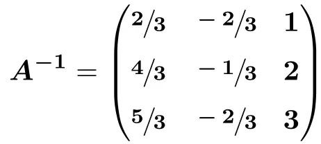
E por fim, operamos:
![\displaystyle A^{-1} = \begin{pmatrix} \sfrac{2}{3} & \sfrac{-2}{3} & \sfrac{3}{3} \\[1.1ex] \sfrac{4}{3} & \sfrac{-1}{3} & \sfrac{6}{3} \\[1.1ex] \sfrac{5}{3} & \sfrac{-2}{3} & \sfrac{9}{3} \end{pmatrix}](https://mathority.org/wp-content/ql-cache/quicklatex.com-41f999c23e7d5ce129b410b9f486983e_l3.png "Rendered by QuickLaTeX.com")
Inverta uma matriz usando o método Gauss:
Para calcular o inverso de uma matriz com o método de Gauss , você deve realizar operações nas linhas de uma matriz (veremos isso mais tarde). Portanto, antes de ver como utilizar o método de Gauss, é importante que você conheça todas as operações que podem ser feitas nas linhas das matrizes:
Transformações de linha permitidas no método gaussiano
- Altere a ordem das linhas da matriz.
Por exemplo, podemos alterar a ordem das linhas 2 e 3 de uma matriz:
![\left( \begin{array}{ccc} 3 & 5 & -2 \\[2ex] -2 & 4 & -1 \\[2ex] 6 & 1 & -3 \end{array} \right) \begin{array}{c} \\[2ex] \xrightarrow{ f_2 \rightarrow f_3}} \\[2ex] \xrightarrow{ f_3 \rightarrow f_2}} \end{array} \left( \begin{array}{ccc} 3 & 5 & -2 \\[2ex] 6 & 1 & -3 \\[2ex] -2 & 4 & -1 \end{array} \right)](https://mathority.org/wp-content/ql-cache/quicklatex.com-1d3f607625afb96bfb250168bd330818_l3.png "Rendered by QuickLaTeX.com")
- Multiplique ou divida todos os termos consecutivos por um número diferente de 0.
Por exemplo, podemos multiplicar a linha 1 por 4 e dividir a linha 3 por 2:
![\left( \begin{array}{ccc} 1 & -2 & 3 \\[2ex] 3 & -1 & 5 \\[2ex] 2 & -4 & -2 \end{array} \right) \begin{array}{c} \xrightarrow{4 f_1} \\[2ex] \\[2ex] \xrightarrow{ f_3 / 2} \end{array} \left( \begin{array}{ccc} 4 & -8 & 12 \\[2ex] 3 & -1 & 5 \\[2ex] 1 & -2 & -1 \end{array} \right)](https://mathority.org/wp-content/ql-cache/quicklatex.com-3cca4df71c23b1f005068a0a93b77dfe_l3.png "Rendered by QuickLaTeX.com")
- Substitua uma linha pela soma da mesma linha mais outra linha multiplicada por um número.
Por exemplo, na matriz a seguir, adicionamos a linha 3 multiplicada por 1 à linha 2:
![\left( \begin{array}{ccc} -1 & -3 & 4 \\[2ex] 2 & 4 & 1 \\[2ex] 1 & -2 & 3 \end{array} \right) \begin{array}{c} \\[2ex] \xrightarrow{f_2 + 1\cdot f_3} \\[2ex] & \end{array} \left( \begin{array}{ccc} -1 & -3 & 4 \\[2ex] 3 & 2 & 4 \\[2ex] 1 & -2 & 3 \end{array} \right)](https://mathority.org/wp-content/ql-cache/quicklatex.com-8ca6644f015dd42ddbf4ab159bd10dec_l3.png "Rendered by QuickLaTeX.com")
Exemplo de cálculo da matriz inversa usando o método Gauss:
Vejamos com um exemplo como aplicar o método Gauss para inverter uma matriz:
- Calcule o inverso da seguinte matriz:
![\displaystyle A = \left( \begin{array}{ccc} 1 & 0 & 1 \\[2ex] 0 & 2 & 1 \\[2ex] 1 & 5 & 4 \end{array} \right)](https://mathority.org/wp-content/ql-cache/quicklatex.com-71553480cefa679dcb8eb98d97e0c717_l3.png "Rendered by QuickLaTeX.com")
A primeira coisa que precisamos fazer é combinar a matriz A e a matriz Identidade em uma única matriz . A matriz A à esquerda e a matriz Identidade à direita:

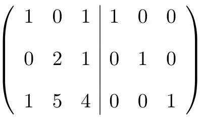
Para calcular a matriz inversa, precisamos converter a matriz esquerda em uma matriz identidade. E, para fazer isso, precisamos aplicar transformações nas linhas até chegarmos lá.
Procederemos por colunas, ou seja, realizaremos operações nas linhas para transformar primeiro os números da primeira coluna, depois os da segunda coluna e por último os da terceira coluna.
Os 1s e 0s da primeira coluna já são adequados, pois a matriz identidade também possui 1 e 0 nessas posições. Portanto, não há necessidade de aplicar uma transformação a essas linhas neste momento.
![\left( \begin{array}{ccc|ccc} \color{blue}\boxed{\color{black}1} & 0 & 1 & 1 & 0 & 0 \\[2ex] \color{blue}\boxed{\color{black}0} & 2 & 1 & 0 & 1 & 0 \\[2ex] 1 & 5 & 4 &0 & 0 & 1 \end{array} \right)](https://mathority.org/wp-content/ql-cache/quicklatex.com-7f51b3a869dde9c1697be9e57fce1548_l3.png "Rendered by QuickLaTeX.com")
No entanto, a matriz identidade tem um 0 no último elemento da primeira coluna, onde agora temos um 1. Portanto, precisamos converter 1 em 0. Para fazer isso, adicionamos a linha 1 multiplicada por – à linha 3.1:

Então se fizermos essa soma teremos a seguinte matriz:
![\left( \begin{array}{ccc|ccc} 1 & 0 & 1 & 1 & 0 & 0 \\[2ex] 0 & 2 & 1 & 0 & 1 & 0 \\[2ex] 1 & 5 & 4 &0 & 0 & 1 \end{array} \right) \begin{array}{c} \\[2ex] \\[2ex] \xrightarrow{f_3 - f_1} \end{array} \left( \begin{array}{ccc|ccc} 1 & 0 & 1 & 1 & 0 & 0 \\[2ex] 0 & 2 & 1 & 0 & 1 & 0 \\[2ex] \color{blue}\boxed{\color{black}0} & 5 & 3 & -1 & 0 & 1 \end{array} \right)](https://mathority.org/wp-content/ql-cache/quicklatex.com-992a31603c2182a97d31ddf787df4f06_l3.png "Rendered by QuickLaTeX.com")
Conseguimos assim transformar 1 em 0.
Agora vamos passar para a segunda coluna da matriz esquerda. O primeiro elemento é 0, o que é bom porque a matriz identidade possui um 0 na mesma posição. No entanto, em vez de 2 deveria haver 1, então dividimos a segunda linha por 2:
![\left( \begin{array}{ccc|ccc} 1 & 0 & 1 & 1 & 0 & 0 \\[2ex] 0 & 2 & 1 & 0 & 1 & 0 \\[2ex] 1 & 5 & 4 &0 & 0 & 1 \end{array} \right) \begin{array}{c} \\[2ex] \xrightarrow{f_2/2}\\[2ex] & \end{array} \left( \begin{array}{ccc|ccc} 1 & 0 & 1 & 1 & 0 & 0 \\[2ex] 0 & \color{blue}\boxed{\color{black}1} & \sfrac{1}{2} & 0 & \sfrac{1}{2} & 0 \\[2ex] 0 & 5 & 3 & -1 & 0 & 1 \end{array} \right)](https://mathority.org/wp-content/ql-cache/quicklatex.com-a86b61ee601f9cd0ff9a70d1a280f887_l3.png "Rendered by QuickLaTeX.com")
Além disso, na segunda coluna também precisamos transformar o 5 em 0. Bem, como o 5 é cinco vezes maior que o 1 na segunda linha, adicionaremos a linha 2 multiplicada por -5 à linha 3:

Portanto, ao realizar esta operação, obtemos a matriz com 0 no último elemento da segunda coluna:
![\left( \begin{array}{ccc|ccc} 1 & 0 & 1 & 1 & 0 & 0 \\[2ex] 0 & 1 & \sfrac{1}{2} & 0 & \sfrac{1}{2} & 0 \\[2ex] 0 & 5 & 3 & -1 & 0 & 1 \end{array} \right) \begin{array}{c} \\[2ex] \\[2ex] \xrightarrow{f_3 - 5f_2} \end{array} \left( \begin{array}{ccc|ccc} 1 & 0 & 1 & 1 & 0 & 0 \\[2ex] 0 & 1 & \sfrac{1}{2} & 0 & \sfrac{1}{2} & 0 \\[2ex] 0 & \color{blue}\boxed{\color{black}0} & \sfrac{1}{2} & -1 & \sfrac{-5}{2} & 1 \end{array} \right)](https://mathority.org/wp-content/ql-cache/quicklatex.com-fcc790f05d73d308cb7d992841ab031a_l3.png "Rendered by QuickLaTeX.com")
Por fim, transformaremos a última coluna da matriz para a esquerda, mas desta vez devemos começar de baixo. É necessário, portanto, transformar o

em 1. Portanto, multiplicamos a última linha por 2:
![\left( \begin{array}{ccc|ccc} 1 & 0 & 1 & 1 & 0 & 0 \\[2ex] 0 & 1 & \sfrac{1}{2} & 0 & \sfrac{1}{2} & 0 \\[2ex] 0 & 0 & \sfrac{1}{2} & -1 & \sfrac{-5}{2} & 1 \end{array} \right)\begin{array}{c} \\[2ex] \\[2ex] \xrightarrow{2f_3} \end{array} \left( \begin{array}{ccc|ccc} 1 & 0 & 1 & 1 & 0 & 0 \\[2ex] 0 & 1 & \sfrac{1}{2} & 0 & \sfrac{1}{2} & 0 \\[2ex] 0 & 0 & \color{blue}\boxed{\color{black}1} & -2 & -5 & 2 \end{array} \right)](https://mathority.org/wp-content/ql-cache/quicklatex.com-69614cae4dd388b6454ffd9b8d63c9a5_l3.png "Rendered by QuickLaTeX.com")
Devemos agora transformar o
restante da última coluna como 0. Porém, desta vez não podemos multiplicar a linha por 2, porque também converteríamos 1 em 2 (quando a matriz identidade tiver 1 nessa posição). Portanto, adicionaremos a linha 3 dividida por -2 à linha 2:

Então fazendo esta operação conseguimos transformar o
em um 0:
![\left( \begin{array}{ccc|ccc} 1 & 0 & 1 & 1 & 0 & 0 \\[2ex] 0 & 1 & \sfrac{1}{2} & 0 & \sfrac{1}{2} & 0 \\[2ex] 0 & 0 & 1 & -2 & -5 & 2 \end{array} \right) \begin{array}{c} \\[2ex] \xrightarrow{f_2-f_3/2} \\[2ex] & \end{array} \left( \begin{array}{ccc|ccc} 1 & 0 & 1 & 1 & 0 & 0 \\[2ex] 0 & 1 & \color{blue}\boxed{\color{black}0} & 1 & 3 & -1 \\[2ex] 0 & 0 & 1 & -2 & -5 & 2 \end{array} \right)](https://mathority.org/wp-content/ql-cache/quicklatex.com-537958a51f67c7602ef121fa2c997ca8_l3.png "Rendered by QuickLaTeX.com")
Por fim, só precisamos transformar o 1 da primeira linha da terceira coluna em 0. A terceira linha também possui um 1 nesta mesma coluna, então adicionaremos a linha 3 multiplicada por -1 à linha 1:

E fazendo esta operação conseguimos converter o 1 em 0:
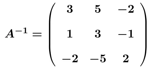
![\ \left( \begin{array}{ccc|ccc} 1 & 0 & 1 & 1 & 0 & 0 \\[2ex] 0 & 1 &0 & 1 & 3 & -1 \\[2ex] 0 & 0 & 1 & -2 & -5 & 2 \end{array} \right) \begin{array}{c} \xrightarrow{f_1-f_3} \\[2ex] \\[2ex] & \end{array} \left( \begin{array}{ccc|ccc} 1 & 0 & \color{blue}\boxed{\color{black}0} & 3 & 5 & -2 \\[2ex] 0 & 1 & 0 & 1 & 3 & -1 \\[2ex] 0 & 0 & 1 & -2 & -5 & 2 \end{array} \right)](https://mathority.org/wp-content/ql-cache/quicklatex.com-8ddd39df6bc92258ba163c65de4fd59f_l3.png "Rendered by QuickLaTeX.com")
Depois de convertermos com sucesso a matriz esquerda em uma matriz identidade, também conhecemos a matriz inversa. Porque a matriz inversa é a matriz que obtemos no lado direito convertendo a matriz esquerda em matriz identidade . O inverso da matriz é portanto:
Exercícios resolvidos sobre matrizes inversas com o método Gauss
Exercício 1
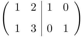
Inverta a seguinte matriz através do método Gauss:
![\displaystyle A=\begin{pmatrix} 1 & 2 \\[1.1ex] 1 & 3 \end{pmatrix}](https://mathority.org/wp-content/ql-cache/quicklatex.com-36886e1ab1007f9a53bdc0dd71a0d15b_l3.png "Rendered by QuickLaTeX.com")
A primeira coisa que precisamos fazer é combinar a matriz A e a matriz Identidade em uma única matriz. A matriz A à esquerda e a matriz identidade à direita:

Agora, para calcular a matriz inversa, precisamos converter a matriz do lado esquerdo em matriz identidade. E, para fazer isso, precisamos aplicar transformações nas linhas até chegarmos lá.
O primeiro termo de todos, 1, já é igual à matriz identidade. Portanto, não há necessidade de aplicar uma transformação à primeira linha neste momento.
No entanto, a matriz identidade tem um 0 no último elemento da primeira coluna, onde agora temos um 1. Portanto, precisamos converter 1 em 0. Para fazer isso, subtraímos a linha 1 da linha 2:
![\left( \begin{array}{cc|cc}1 & 2 & 1 & 0 \\[1.5ex] 1 & 3 & 0 & 1\end{array} \right) \begin{array}{c} \\[1.5ex] \xrightarrow{f_2 - f_1} \end{array} \left( \begin{array}{cc|cc} 1 & 2 & 1 & 0 \\[1.5ex] 0 & 1 & -1 & 1\end{array} \right)](https://mathority.org/wp-content/ql-cache/quicklatex.com-247d8605795c43e79b5d7742854cfe6d_l3.png "Rendered by QuickLaTeX.com")
Passamos para a segunda coluna: 1 abaixo é bom. Mas não o 2 acima, já que a matriz identidade tem 0 nessa posição. Portanto, para converter 2 em 0, da linha 1 subtraímos a linha 2 multiplicada por 2:
![\left( \begin{array}{cc|cc} 1 & 2 & 1 & 0 \\[1.5ex] 0 & 1 & -1 & 1 \end{array} \right) \begin{array}{c} \xrightarrow{f_1 - 2f_2} \\[1.5ex] & \end{array} \left( \begin{array}{cc|cc} 1 & 0 & 3 & -2 \\[1.5ex] 0 & 1 & -1 & 1 \end{array} \right)](https://mathority.org/wp-content/ql-cache/quicklatex.com-173a7bdb55ba058e5ae16d1fd8e91564_l3.png "Rendered by QuickLaTeX.com")
A matriz inversa é a matriz que obtemos do lado direito após converter a matriz da esquerda em uma matriz identidade. E agora temos a matriz identidade no lado esquerdo. A matriz inversa é portanto:
![\bm{A^{-1}= \left(} \begin{array}{cc} \bm{3} & \bm{-2} \\[1.5ex] \bm{-1} & \bm{1} \end{array}\bm{ \right)}](https://mathority.org/wp-content/ql-cache/quicklatex.com-98896d28465c9e1402e1c443375d93fe_l3.png "Rendered by QuickLaTeX.com")
Exercício 2
Inverta a seguinte matriz com o procedimento gaussiano:
![\displaystyle A=\begin{pmatrix} 1 & 1 & -4 \\[1.1ex] 0 & 3 & 2 \\[1.1ex] 0 & 1 & 1 \end{pmatrix}](https://mathority.org/wp-content/ql-cache/quicklatex.com-7ae5ba4a92a5ddc00ddf5b11775edafd_l3.png "Rendered by QuickLaTeX.com")
Primeiro, colocamos a matriz A e a matriz Identidade em uma única matriz:
![\left( \begin{array}{ccc|ccc} 1 & 1 & -4 & 1 & 0 & 0 \\[2ex] 0 & 3 & 2 & 0 & 1 & 0 \\[2ex] 0 & 1 & 1 & 0 & 0 & 1 \end{array} \right)](https://mathority.org/wp-content/ql-cache/quicklatex.com-81db2ef94d2db597cebb4c0c77685526_l3.png "Rendered by QuickLaTeX.com")
Agora precisamos transformar as linhas até convertermos a matriz esquerda em uma matriz identidade.
A primeira coluna da matriz esquerda já é igual à primeira coluna da matriz identidade. Portanto, não é necessário modificar nenhum dos seus números.
No entanto, a matriz identidade tem um 1 no segundo elemento da segunda coluna, onde agora existe um 3. Devemos, portanto, converter o 3 em 1. Para fazer isso, da linha 2 subtraímos a linha 3 multiplicada por 2:
![\left( \begin{array}{ccc|ccc} 1 & 1 & -4 & 1 & 0 & 0 \\[2ex] 0 & 3 & 2 & 0 & 1 & 0 \\[2ex] 0 & 1 & 1 & 0 & 0 & 1 \end{array} \right) \begin{array}{c} \\[2ex] \xrightarrow{f_2 - 2f_3} \\[2ex] & \end{array} \left( \begin{array}{ccc|ccc} 1 & 1 & 4 & 1 & 0 & 0 \\[2ex] 0 & 1 & 0 & 0 & 1 & -2 \\[2ex] 0 & 1 & 1 & 0 & 0 & 1 \end{array} \right)](https://mathority.org/wp-content/ql-cache/quicklatex.com-bfd7cb4d4b81a75038807eb28393a83e_l3.png "Rendered by QuickLaTeX.com")
A matriz identidade tem um 0 no último elemento da segunda coluna, onde agora existe um 1. Devemos, portanto, converter o 1 em 0. Para fazer isso, subtraímos a linha 2 da linha 3:
![\left( \begin{array}{ccc|ccc} 1 & 1 & -4 & 1 & 0 & 0 \\[2ex] 0 & 1 & 0 & 0 & 1 & -2 \\[2ex] 0 & 1 & 1 & 0 & 0 & 1 \end{array} \right) \begin{array}{c} \\[2ex] \\[2ex] \xrightarrow{f_3 - f_2} \end{array} \left( \begin{array}{ccc|ccc} 1 & 1 & -4 & 1 & 0 & 0 \\[2ex] 0 & 1 & 0 & 0 & 1 & -2 \\[2ex] 0 & 0 & 1 & 0 & -1 & 3 \end{array} \right)](https://mathority.org/wp-content/ql-cache/quicklatex.com-932479e2f574c19ad7906d3d20e52ad0_l3.png "Rendered by QuickLaTeX.com")
A matriz identidade tem um 0 no primeiro elemento da segunda coluna, onde agora existe um 1. Devemos, portanto, converter 1 em 0. Para fazer isso, subtraímos a linha 2 da linha 1:
![\left( \begin{array}{ccc|ccc} 1 & 1 & -4 & 1 & 0 & 0 \\[2ex] 0 & 1 & 0 & 0 & 1 & -2 \\[2ex] 0 & 0 & 1 & 0 & -1 & 3 \end{array} \right) \begin{array}{c} \xrightarrow{f_1 - f_2} \\[2ex] \\[2ex] & \end{array} \left( \begin{array}{ccc|ccc}1 & 0 & -4 & 1 & -1 & 2 \\[2ex] 0 & 1 & 0 & 0 & 1 & -2 \\[2ex] 0 & 0 & 1 & 0 & -1 & 3 \end{array} \right)](https://mathority.org/wp-content/ql-cache/quicklatex.com-566e1453aab03f9792cb281e4c88a68c_l3.png "Rendered by QuickLaTeX.com")
Tudo o que precisamos fazer agora é converter -4 em 0. Para fazer isso, adicionamos a linha 3 multiplicada por 4 à linha 1:
![\left( \begin{array}{ccc|ccc} 1 & 0 & -4 & 1 & -1 & 2 \\[2ex] 0 & 1 & 0 & 0 & 1 & -2 \\[2ex] 0 & 0 & 1 & 0 & -1 & 3\end{array} \right) \begin{array}{c} \xrightarrow{f_1 + 4f_3} \\[2ex] \\[2ex] & \end{array} \left( \begin{array}{ccc|ccc}1 & 0 & 0 & 1 & -5 & 14 \\[2ex] 0 & 1 & 0 & 0 & 1 & -2 \\[2ex] 0 & 0 & 1 & 0 & -1 & 3 \end{array} \right)](https://mathority.org/wp-content/ql-cache/quicklatex.com-6f98a9cabeb101602dd11aa73516b998_l3.png "Rendered by QuickLaTeX.com")
Já obtivemos a matriz identidade do lado esquerdo. A matriz inversa é portanto:
![\bm{A^{-1}= \left( } \begin{array}{ccc} \bm{1} & \bm{-5} & \bm{14} \\[2ex] \bm{0} & \bm{1} & \bm{-2} \\[2ex] \bm{0} & \bm{-1 }& \bm{3} \end{array} \bm{ \right)}](https://mathority.org/wp-content/ql-cache/quicklatex.com-e43ce6a7061f0339bd5d44b83afec07f_l3.png "Rendered by QuickLaTeX.com")
Exercício 3
Inverta a seguinte matriz usando o método Gaussiano:
![\displaystyle A=\begin{pmatrix} 1 & 2 & 1 \\[1.1ex] 0 & 1 & 0 \\[1.1ex] 2 & 0 & 3 \end{pmatrix}](https://mathority.org/wp-content/ql-cache/quicklatex.com-f02b0186690e68baaa9a630db2c870db_l3.png "Rendered by QuickLaTeX.com")
Antes de começarmos a operar, precisamos colocar a matriz A e a matriz Identidade em uma única matriz:
![\left( \begin{array}{ccc|ccc} 1 & 2 & 1 & 1 & 0 & 0 \\[2ex] 0 & 1 & 0 & 0 & 1 & 0 \\[2ex] 2 & 0 & 3 & 0 & 0 & 1 \end{array} \right)](https://mathority.org/wp-content/ql-cache/quicklatex.com-aa6dc5af82076e22b1d0cf7ea16d748b_l3.png "Rendered by QuickLaTeX.com")
Devemos agora converter a matriz esquerda em uma matriz identidade operando nas linhas.
Os dois primeiros elementos da primeira coluna já são iguais aos da matriz identidade. Por conseguinte, não é necessário alterar estes valores.
Mas a matriz identidade tem um 0 no terceiro elemento da primeira coluna, onde agora existe um 2. Devemos, portanto, converter o 2 em 0. Para fazer isso, da linha 3 subtraímos a linha 1 multiplicada por 2:
![\left( \begin{array}{ccc|ccc}1 & 2 & 1 & 1 & 0 & 0 \\[2ex] 0 & 1 & 0 & 0 & 1 & 0 \\[2ex] 2 & 0 & 3 & 0 & 0 & 1 \end{array} \right) \begin{array}{c} \\[2ex] \\[2ex] \xrightarrow{f_3 - 2f_1} \end{array} \left( \begin{array}{ccc|ccc} 1 & 2 & 1 & 1 & 0 & 0 \\[2ex] 0 & 1 & 0 & 0 & 1 & 0 \\[2ex] 0 & -4 & 1 & -2 & 0 & 1 \end{array} \right)](https://mathority.org/wp-content/ql-cache/quicklatex.com-680a314b8cc900e01886291af12145e4_l3.png "Rendered by QuickLaTeX.com")
A matriz identidade tem um 0 no primeiro elemento da segunda coluna, onde agora existe um 2. Devemos, portanto, converter o 2 em 0. Para fazer isso, da linha 1 subtraímos a linha 2 multiplicada por 2:
![\left( \begin{array}{ccc|ccc} 1 & 2 & 1 & 1 & 0 & 0 \\[2ex] 0 & 1 & 0 & 0 & 1 & 0 \\[2ex] 0 & -4 & 1 & -2 & 0 & 1 \end{array} \right) \begin{array}{c} \xrightarrow{f_1 -2f_2} \\[2ex] \\[2ex] & \end{array} \left( \begin{array}{ccc|ccc} 1 & 0 & 1 & 1 & -2 & 0\\[2ex] 0 & 1 & 0 & 0 & 1 & 0 \\[2ex] 0 & -4 & 1 & -2 & 0 & 1 \end{array} \right)](https://mathority.org/wp-content/ql-cache/quicklatex.com-f87cbc594287f7ea4938091878562b4c_l3.png "Rendered by QuickLaTeX.com")
A matriz identidade possui 0 no último elemento da segunda coluna, onde agora existe -4. Devemos, portanto, converter -4 em 0. Para fazer isso, adicionamos a linha 2 multiplicada por 4 à linha 3:
![\left( \begin{array}{ccc|ccc} 1 & 0 & 1 & 1 & -2 & 0\\[2ex] 0 & 1 & 0 & 0 & 1 & 0 \\[2ex] 0 & -4 & 1 & -2 & 0 & 1 \end{array} \right) \begin{array}{c} \\[2ex] \\[2ex] \xrightarrow{f_3 +4f_2} \end{array} \left( \begin{array}{ccc|ccc} 1 & 0 & 1 & 1 & -2 & 0\\[2ex] 0 & 1 & 0 & 0 & 1 & 0 \\[2ex] 0 & 0 & 1 & -2 & 4 & 1 \end{array} \right)](https://mathority.org/wp-content/ql-cache/quicklatex.com-b8cf2c3878d2d35656953a55bb3baf94_l3.png "Rendered by QuickLaTeX.com")
Tudo o que precisamos fazer agora é converter o primeiro elemento da terceira coluna em 0. Para fazer isso, adicionamos a linha 3 multiplicada por -1 à linha 1:
![\left( \begin{array}{ccc|ccc}1 & 0 & 1 & 1 & -2 & 0\\[2ex] 0 & 1 & 0 & 0 & 1 & 0 \\[2ex] 0 & 0 & 1 & -2 & 4 & 1 \end{array} \right) \begin{array}{c} \xrightarrow{f_1 - f_3} \\[2ex] \\[2ex] & \end{array} \left( \begin{array}{ccc|ccc}1 & 0 & 0 & 3 & -6 & -1\\[2ex] 0 & 1 & 0 & 0 & 1 & 0 \\[2ex] 0 & 0 & 1 & -2 & 4 & 1 \end{array} \right)](https://mathority.org/wp-content/ql-cache/quicklatex.com-aac851b05c2dc25af3d7b9ecc622c9f6_l3.png "Rendered by QuickLaTeX.com")
Já percebemos que a matriz à esquerda é a matriz identidade. Então o inverso da matriz
Leste:
![\bm{A^{-1}= \left( } \begin{array}{ccc} \bm{3} & \bm{-6} & \bm{-1} \\[2ex] \bm{0} & \bm{1} & \bm{0} \\[2ex] \bm{-2} & \bm{4}& \bm{1} \end{array} \bm{ \right)}](https://mathority.org/wp-content/ql-cache/quicklatex.com-161fbe4a4d4dcc4fc503b6e3a9e0bfeb_l3.png "Rendered by QuickLaTeX.com")
Exercício 4
Inverta a seguinte matriz usando o método Gaussiano:
![\displaystyle A=\begin{pmatrix} 1 & -2 & 0 \\[1.1ex] 1 & 2 & 2 \\[1.1ex] 0 & 3 & 2 \end{pmatrix}](https://mathority.org/wp-content/ql-cache/quicklatex.com-47ad7ccd6aafab72255c96f2bc9148a2_l3.png "Rendered by QuickLaTeX.com")
A primeira coisa que precisamos fazer é juntar a matriz A e a matriz Identidade em uma única matriz:
![\left( \begin{array}{ccc|ccc}1 & -2 & 0 & 1 & 0 & 0 \\[2ex] 1 & 2 & 2 & 0 & 1 & 0 \\[2ex] 0 & 3 & 2 & 0 & 0 & 1 \end{array} \right)](https://mathority.org/wp-content/ql-cache/quicklatex.com-a832ceb9f09dfa88238c570b46b74d92_l3.png "Rendered by QuickLaTeX.com")
Devemos agora converter a matriz do lado esquerdo em uma matriz identidade aplicando operações sobre linhas.
O primeiro elemento da primeira coluna já é igual ao da matriz identidade. Portanto, não é necessário alterá-lo.
No entanto, a matriz identidade tem um 0 no segundo elemento da primeira coluna, onde agora existe um 1. Devemos, portanto, converter o 1 em 0. Para fazer isso, subtraímos a linha 1 da linha 2:
![\left( \begin{array}{ccc|ccc}1 & -2 & 0 & 1 & 0 & 0 \\[2ex] 1 & 2 & 2 & 0 & 1 & 0 \\[2ex] 0 & 3 & 2 & 0 & 0 & 1 \end{array} \right) \begin{array}{c} \\[2ex] \xrightarrow{f_2 - f_1} \\[2ex] & \end{array} \left( \begin{array}{ccc|ccc} 1 & -2 & 0 & 1 & 0 & 0 \\[2ex] 0 & 4 & 2 & -1 & 1 & 0 \\[2ex] 0 & 3 & 2 & 0 & 0 & 1 \end{array} \right)](https://mathority.org/wp-content/ql-cache/quicklatex.com-83933b5a2315a4dcbc770bf92bf3831b_l3.png "Rendered by QuickLaTeX.com")
Passamos para a segunda coluna: primeiro transformamos o 4 em 1 dividindo a segunda linha por 4:
![\left( \begin{array}{ccc|ccc} 1 & -2 & 0 & 1 & 0 & 0 \\[2ex] 0 & 4 & 2 & -1 & 1 & 0 \\[2ex] 0 & 3 & 2 & 0 & 0 & 1\end{array} \right) \begin{array}{c} \\[2ex] \xrightarrow{f_2/4} \\[2ex] & \end{array} \left( \begin{array}{ccc|ccc} 1 & -2 & 0 & 1 & 0 & 0 \\[2ex] 0 & 1 & \sfrac{2}{4} & \sfrac{-1}{4} & \sfrac{1}{4} & 0 \\[2ex] 0 & 3 & 2 & 0 & 0 & 1 \end{array} \right)](https://mathority.org/wp-content/ql-cache/quicklatex.com-298984c72a249e2b5c98740cc0c1a11e_l3.png "Rendered by QuickLaTeX.com")
A matriz identidade possui 0 no primeiro elemento da segunda coluna, onde agora existe -2. Devemos, portanto, converter -2 em 0. Para fazer isso, adicionamos a linha 2 multiplicada por 2 à linha 1:

![\left( \begin{array}{ccc|ccc} 1 & -2 & 0 & 1 & 0 & 0 \\[2ex] 0 & 1 & \sfrac{2}{4} & \sfrac{-1}{4} & \sfrac{1}{4} & 0 \\[2ex] 0 & 3 & 2 & 0 & 0 & 1\end{array} \right) \begin{array}{c} \xrightarrow{f_1 +2f_2} \\[2ex] \\[2ex] & \end{array} \left( \begin{array}{ccc|ccc} 1 & 0 & 1 & \sfrac{2}{4} & \sfrac{2}{4} & 0 \\[2ex] 0 & 1 & \sfrac{2}{4} & \sfrac{-1}{4} & \sfrac{1}{4} & 0 \\[2ex] 0 & 3 & 2 & 0 & 0 & 1 \end{array} \right)](https://mathority.org/wp-content/ql-cache/quicklatex.com-3dfcdcb586eed87861b3ac0ea46bea2f_l3.png "Rendered by QuickLaTeX.com")
A matriz identidade tem um 0 no último elemento da segunda coluna, onde agora existe um 3. Devemos, portanto, converter o 3 em 0. Para fazer isso, da linha 3 subtraímos a linha 2 multiplicada por 3:

![\left( \begin{array}{ccc|ccc} 1 & 0 & 1 & \sfrac{2}{4} & \sfrac{2}{4} & 0 \\[2ex] 0 & 1 & \sfrac{2}{4} & \sfrac{-1}{4} & \sfrac{1}{4} & 0 \\[2ex] 0 & 3 & 2 & 0 & 0 & 1 \end{array} \right) \begin{array}{c} \\[2ex] \\[2ex] \xrightarrow{f_3 -3f_2} \end{array} \left( \begin{array}{ccc|ccc} 1 & 0 & 1 & \sfrac{2}{4} & \sfrac{2}{4} & 0 \\[2ex] 0 & 1 & \sfrac{2}{4} & \sfrac{-1}{4} & \sfrac{1}{4} & 0 \\[2ex] 0 & 0 &\sfrac{2}{4} & \sfrac{3}{4} & \sfrac{-3}{4} & 1 \end{array} \right)](https://mathority.org/wp-content/ql-cache/quicklatex.com-94ed5a1b9cf1db0bfb99ce79d0a6d36b_l3.png "Rendered by QuickLaTeX.com")
Passamos para a terceira coluna: devemos transformar a última

em 1. Para fazer isso, multiplicamos a terceira linha por 2:
![\left( \begin{array}{ccc|ccc} 1 & 0 & 1 & \sfrac{2}{4} & \sfrac{2}{4} & 0 \\[2ex] 0 & 1 & \sfrac{2}{4} & \sfrac{-1}{4} & \sfrac{1}{4} & 0 \\[2ex] 0 & 0 &\sfrac{2}{4} & \sfrac{3}{4} & \sfrac{-3}{4} & 1 \end{array} \right) \begin{array}{c} \\[2ex] \\[2ex] \xrightarrow{2f_3 } \end{array} \left( \begin{array}{ccc|ccc} 1 & 0 & 1 & \sfrac{2}{4} & \sfrac{2}{4} & 0 \\[2ex] 0 & 1 & \sfrac{2}{4} & \sfrac{-1}{4} & \sfrac{1}{4} & 0 \\[2ex] 0 & 0 & 1 & \sfrac{6}{4} & \sfrac{-6}{4} & 2 \end{array} \right)](https://mathority.org/wp-content/ql-cache/quicklatex.com-a8134938726d3b48fe3d7d789260b128_l3.png "Rendered by QuickLaTeX.com")
A matriz identidade possui um 0 no segundo elemento da última coluna. É necessário, portanto, converter o
em 0. Para fazer isso, da linha 2 subtraímos a linha 3 dividida por 2:

![\left( \begin{array}{ccc|ccc} 1 & 0 & 1 & \sfrac{2}{4} & \sfrac{2}{4} & 0 \\[2ex] 0 & 1 & \sfrac{2}{4} & \sfrac{-1}{4} & \sfrac{1}{4} & 0 \\[2ex] 0 & 0 & 1 & \sfrac{6}{4} & \sfrac{-6}{4} & 2 \end{array} \right) \begin{array}{c} \\[2ex] \xrightarrow{f_2-f_3/2 } \\[2ex] & \end{array} \left( \begin{array}{ccc|ccc} 1 & 0 & 1 & \sfrac{2}{4} & \sfrac{2}{4} & 0 \\[2ex] 0 & 1 & 0 & -1 & 1 & -1 \\[2ex] 0 & 0 & 1 & \sfrac{6}{4} & \sfrac{-6}{4} & 2 \end{array} \right)](https://mathority.org/wp-content/ql-cache/quicklatex.com-8b91b71183a50e41e9be5c7305f8cf3e_l3.png "Rendered by QuickLaTeX.com")
Tudo o que precisamos fazer agora é converter o primeiro elemento da terceira coluna em 0. Para fazer isso, subtraímos a linha 3 da linha 1:

![\left( \begin{array}{ccc|ccc}1 & 0 & 1 & \sfrac{2}{4} & \sfrac{2}{4} & 0 \\[2ex] 0 & 1 & 0 & -1 & 1 & -1 \\[2ex] 0 & 0 & 1 & \sfrac{6}{4} & \sfrac{-6}{4} & 2 \end{array} \right) \begin{array}{c} \xrightarrow{f_1-f_3 } \\[2ex] \\[2ex] & \end{array} \left( \begin{array}{ccc|ccc} 1 & 0 & 0 & -1 & 2 & -2 \\[2ex] 0 & 1 & 0 & -1 & 1 & -1 \\[2ex] 0 & 0 & 1 & \sfrac{6}{4} & \sfrac{-6}{4} & 2 \end{array} \right)](https://mathority.org/wp-content/ql-cache/quicklatex.com-2023374b9885dd33fe4d3c12e5a4de59_l3.png "Rendered by QuickLaTeX.com")
A matriz inversa é portanto:
![A^{-1}= \left( \begin{array}{ccc} -1 & 2 & -2 \\[2ex] -1 & 1 & -1 \\[2ex] \sfrac{6}{4} &\sfrac{-6}{4} & 2 \end{array} \bm{ \right)}](https://mathority.org/wp-content/ql-cache/quicklatex.com-0854e7cb80ba561b6e0c724a9a9b5fff_l3.png "Rendered by QuickLaTeX.com")
Finalmente, as frações da matriz inversa podem ser simplificadas:
![\bm{A^{-1}= \left( } \begin{array}{ccc} \bm{-1} & \bm{2} & \bm{-2} \\[2ex] \bm{-1} & \bm{1} & \bm{-1} \\[2ex] \sfrac{\bm{3}}{\bm{2}} &\sfrac{\bm{-3}}{\bm{2}} & \bm{2} \end{array} \bm{ \right)}](https://mathority.org/wp-content/ql-cache/quicklatex.com-6c7ef6b6cdca2f4a808ed9457bde3b3f_l3.png "Rendered by QuickLaTeX.com")
Propriedades da matriz inversa
A matriz inversa possui as seguintes características:
- O inverso de uma matriz é único .
- O inverso da matriz inversa é a matriz original:

- O inverso da multiplicação de duas matrizes é igual ao produto dos inversos das matrizes, mas mudando sua ordem.

- Transpor uma matriz e depois fazer a inversa da matriz é como primeiro fazer a inversão da matriz e depois transpô-la.

- Para resolver o determinante do inverso de uma matriz podemos calcular o determinante da matriz e depois fazer o seu inverso, pois as duas operações dão o mesmo resultado.

Fórmula para calcular rapidamente o inverso de uma matriz 2×2
Como vimos, qualquer matriz pode ser invertida pelo método dos determinantes ou pelo método de Gauss. Mas, separadamente, existe também uma fórmula para encontrar muito rapidamente o inverso de uma matriz 2×2 :

Como você pode ver, inverter uma matriz 2×2 é simples: basta resolver o determinante da matriz

, alterne a posição dos elementos da diagonal principal e altere o sinal dos elementos da diagonal secundária.
Exemplo de como obter uma matriz inversa 2 × 2 com a fórmula
Calcule o inverso da seguinte matriz quadrada 2 × 2:
![\displaystyle A = \begin{pmatrix} 3 & 5 \\[1.1ex] -2 & -4 \end{pmatrix}](https://mathority.org/wp-content/ql-cache/quicklatex.com-599baee27c05b5610a8714363e1260eb_l3.png "Rendered by QuickLaTeX.com")
O determinante da matriz A é:
![\displaystyle \begin{aligned}\begin{vmatrix}A\end{vmatrix} = \begin{vmatrix} 3 & 5 \\[1.1ex] -2 & -4 \end{vmatrix} & = 3 \cdot (-4)- (-2) \cdot 5 \\ & = -12-(-10) \\[2ex] & =-12+10\\[2ex] &=-2\end{aligned}](https://mathority.org/wp-content/ql-cache/quicklatex.com-ab99f7b87d01c670a8598df6364ab58f_l3.png "Rendered by QuickLaTeX.com")
Agora aplicamos a fórmula da matriz inversa :
![\displaystyle A = \begin{pmatrix} a & b \\[1.1ex] c & d \end{pmatrix}\longrightarrow A^{-1} = \cfrac{1}{|A|} \begin{pmatrix} d & -b \\[1.1ex] -c & a \end{pmatrix}](https://mathority.org/wp-content/ql-cache/quicklatex.com-7d5308484309da4485a3d9b92af86e7d_l3.png "Rendered by QuickLaTeX.com")
![\displaystyle A = \begin{pmatrix} 3 & 5 \\[1.1ex] -2 & -4 \end{pmatrix}\longrightarrow A^{-1} = \cfrac{1}{-2} \begin{pmatrix} -4 & -5 \\[1.1ex] 2 & 3 \end{pmatrix}](https://mathority.org/wp-content/ql-cache/quicklatex.com-68fd6e830b576af8abf55be1e11fbafb_l3.png "Rendered by QuickLaTeX.com")
E multiplicamos a matriz pela fração:
![\displaystyle A^{-1} =\begin{pmatrix} \cfrac{-4}{-2} & \cfrac{-5}{-2} \\[3ex] \cfrac{2}{-2} & \cfrac{3}{-2} \end{pmatrix}](https://mathority.org/wp-content/ql-cache/quicklatex.com-41da8ef6bef1d339337717ed4ad86ae5_l3.png "Rendered by QuickLaTeX.com")
A matriz invertida A é portanto:
![\displaystyle \bm{A^{-1} =}\begin{pmatrix} \bm{2} & \cfrac{\bm{5}}{\bm{2}} \\[3ex] \bm{-1} & \bm{-}\cfrac{\bm{3}}{\bm{2}} \end{pmatrix}](https://mathority.org/wp-content/ql-cache/quicklatex.com-29da2a64f6da927857de112ca8363ba5_l3.png "Rendered by QuickLaTeX.com")
Como você pode ver, inverter uma matriz com esta fórmula é muito mais rápido, mas só pode ser usada em matrizes de dimensão 2×2.
Exercícios resolvidos de matrizes inversas 2×2 com a fórmula
Exercício 1
Inverta a seguinte matriz de dimensão 2×2:
![\displaystyle A=\begin{pmatrix} 2 & 5 \\[1.1ex] 1 & 3 \end{pmatrix}](https://mathority.org/wp-content/ql-cache/quicklatex.com-dc06e21fc1c3c54f9b3fc0dcd4912a8f_l3.png "Rendered by QuickLaTeX.com")
O determinante da matriz A é:
![\displaystyle \begin{aligned}\begin{vmatrix}A\end{vmatrix} = \begin{vmatrix} 2 & 5 \\[1.1ex] 1 & 3 \end{vmatrix} & = 2 \cdot 3- 1 \cdot 5 \\ & = 6-5 \\[2ex] & =1\end{aligned}](https://mathority.org/wp-content/ql-cache/quicklatex.com-1b0ae510ea7a336cbe5ea56a554da719_l3.png "Rendered by QuickLaTeX.com")
Agora aplicamos a fórmula para encontrar a matriz inversa:
![\displaystyle A=\begin{pmatrix} 2 & 5 \\[1.1ex] 1 & 3 \end{pmatrix} \longrightarrow A^{-1} = \cfrac{1}{1} \begin{pmatrix} 3 & -5 \\[1.1ex] -1 & 2 \end{pmatrix}](https://mathority.org/wp-content/ql-cache/quicklatex.com-b8f18178c829fd38360a04a947d52017_l3.png "Rendered by QuickLaTeX.com")
O inverso da matriz A é, portanto:
![\displaystyle \bm{A^{-1} =}\begin{pmatrix} \bm{3} & \bm{-5} \\[1.1ex] \bm{-1} & \bm{2} \end{pmatrix}](https://mathority.org/wp-content/ql-cache/quicklatex.com-237fe82cd91972f667f6751fa4735534_l3.png "Rendered by QuickLaTeX.com")
Exercício 2
Calcule o inverso da seguinte matriz de ordem 2:
![\displaystyle A=\begin{pmatrix} 2 & 6 \\[1.1ex] -1 & -2 \end{pmatrix}](https://mathority.org/wp-content/ql-cache/quicklatex.com-f2289d1c5c9aeb87016f719305d900a7_l3.png "Rendered by QuickLaTeX.com")
O determinante da matriz A é:
![\displaystyle \begin{aligned}\begin{vmatrix}A\end{vmatrix} = \begin{vmatrix} 2 & 6 \\[1.1ex] -1 & -2 \end{vmatrix} & = 2 \cdot (-2)- (-1) \cdot 6 \\ & = -4-(-6) \\[2ex] & =-4+6 \\[2ex] & =2\end{aligned}](https://mathority.org/wp-content/ql-cache/quicklatex.com-a3fef2cc00702131123994cc588bf7ea_l3.png "Rendered by QuickLaTeX.com")
Agora aplicamos a fórmula para resolver a matriz inversa de dimensão 2×2:
![\displaystyle A=\begin{pmatrix} 2 & 6 \\[1.1ex] -1 & -2 \end{pmatrix} \longrightarrow A^{-1} = \cfrac{1}{2} \begin{pmatrix} -2 & -6 \\[1.1ex] 1 & 2 \end{pmatrix}](https://mathority.org/wp-content/ql-cache/quicklatex.com-2de7166a0cf59e0f8c5b7750e1947f04_l3.png "Rendered by QuickLaTeX.com")
E por fim, fazemos a multiplicação:
![\displaystyle A^{-1} = \begin{pmatrix} \cfrac{-2}{2} & \cfrac{-6}{2} \\[3ex] \cfrac{1}{2} & \cfrac{2}{2} \end{pmatrix}](https://mathority.org/wp-content/ql-cache/quicklatex.com-f6a5973078468914beb4bd4d85a40331_l3.png "Rendered by QuickLaTeX.com")
![\displaystyle \bm{A^{-1} =}\begin{pmatrix} \bm{-1} & \bm{-3} \\[2ex] \cfrac{\bm{1}}{\bm{2}} & \bm{1} \end{pmatrix}](https://mathority.org/wp-content/ql-cache/quicklatex.com-a540a077ee9a24da96fa988410aef429_l3.png "Rendered by QuickLaTeX.com")
Exercício 3
Inverta a seguinte matriz 2×2:
![\displaystyle A=\begin{pmatrix} 4 & 1 \\[1.1ex] 5 & 2 \end{pmatrix}](https://mathority.org/wp-content/ql-cache/quicklatex.com-36e230a808c42411a9cfd2d9eb44543d_l3.png "Rendered by QuickLaTeX.com")
O determinante da matriz A é:
![\displaystyle \begin{aligned}\begin{vmatrix}A\end{vmatrix} = \begin{vmatrix} 4 & 1 \\[1.1ex] 5 & 2\end{vmatrix} & = 4 \cdot 2 - 5 \cdot 1 \\ & = 8-5 \\[2ex] & =3\end{aligned}](https://mathority.org/wp-content/ql-cache/quicklatex.com-e7a6c5ef316ae51b43c90863c6245780_l3.png "Rendered by QuickLaTeX.com")
Agora aplicamos a fórmula para calcular a matriz inversa de dimensão 2×2:
![\displaystyle A=\begin{pmatrix} 4 & 1 \\[1.1ex] 5 & 2 \end{pmatrix} \longrightarrow A^{-1} = \cfrac{1}{3} \begin{pmatrix} 2 & -1 \\[1.1ex] -5 & 4 \end{pmatrix}](https://mathority.org/wp-content/ql-cache/quicklatex.com-e2f359bd166c295b869a8cf04d927097_l3.png "Rendered by QuickLaTeX.com")
E por fim, fazemos o produto entre a fração e a matriz:
![\displaystyle A^{-1} = \begin{pmatrix} \cfrac{\bm{2}}{\bm{3}} & \bm{-}\cfrac{\bm{1}}{\bm{3}} \\[3ex] \bm{-}\cfrac{\bm{5}}{\bm{3}} & \cfrac{\bm{4}}{\bm{3}} \end{pmatrix}](https://mathority.org/wp-content/ql-cache/quicklatex.com-6a02ea2e547dcc21081ae80df407a4e0_l3.png "Rendered by QuickLaTeX.com")
Exercício 4
Encontre o inverso da seguinte matriz de segunda ordem:
![\displaystyle A=\begin{pmatrix} -2 & 5 \\[1.1ex] -3 & 10 \end{pmatrix}](https://mathority.org/wp-content/ql-cache/quicklatex.com-422fcd6f391a2682e4b546c9e9c05b55_l3.png "Rendered by QuickLaTeX.com")
O determinante da matriz A é:
![\displaystyle \begin{aligned}\begin{vmatrix}A\end{vmatrix} = \begin{vmatrix} -2 & 5 \\[1.1ex] -3 & 10\end{vmatrix} & = (-2) \cdot 10- (-3) \cdot 5 \\ & = -20-(-15) \\[2ex] & =-20+15 \\[2ex] & =-5\end{aligned}](https://mathority.org/wp-content/ql-cache/quicklatex.com-9e9997751e16d3b976454be828cb914d_l3.png "Rendered by QuickLaTeX.com")
Agora aplicamos a fórmula para criar a matriz inversa de dimensão 2×2:
![\displaystyle A=\begin{pmatrix} -2 & 5 \\[1.1ex] -3 & 10\end{pmatrix} \longrightarrow A^{-1} = \cfrac{1}{-5} \begin{pmatrix} 10 & -5 \\[1.1ex] 3 & -2 \end{pmatrix}](https://mathority.org/wp-content/ql-cache/quicklatex.com-7c0c614039614bd9125b2920da8698eb_l3.png "Rendered by QuickLaTeX.com")
E por fim, fazemos a multiplicação:
![\displaystyle A^{-1} = \begin{pmatrix} \cfrac{10}{-5} & \cfrac{-5}{-5} \\[3ex] \cfrac{3}{-5} & \cfrac{-2}{-5} \end{pmatrix}](https://mathority.org/wp-content/ql-cache/quicklatex.com-edb1dfc870b3045eaefc1716a80e2ca2_l3.png "Rendered by QuickLaTeX.com")
![\displaystyle \bm{A^{-1} =}\begin{pmatrix} \bm{-2} & \bm{1} \\[2ex] \bm{-}\cfrac{\bm{3}}{\bm{5}} & \cfrac{\bm{2}}{\bm{5}} \ \end{pmatrix}](https://mathority.org/wp-content/ql-cache/quicklatex.com-5c49e161c701254cfbe20353c11980eb_l3.png "Rendered by QuickLaTeX.com")
Resolva um sistema de equações com a matriz inversa
É difícil apreciar as aplicações reais da inversa de uma matriz. Na verdade, você provavelmente está se perguntando… para que serve a matriz inversa? É realmente usado para alguma coisa?
Bom, um dos usos da matriz inversa é resolver sistemas de equações lineares . E sim, embora possam parecer dois conceitos muito diferentes, é possível encontrar a solução de um sistema de equações invertendo uma matriz.
Vamos ver com um exemplo como isso é feito:
- Calcule a solução do seguinte sistema de equações com a matriz inversa:
![\left. \begin{array}{r} x+3y=5 \\[2ex] 2x+4y=6 \end{array} \right\}](https://mathority.org/wp-content/ql-cache/quicklatex.com-200c0f994f86752e7d650621a0d4100f_l3.png "Rendered by QuickLaTeX.com")
Em primeiro lugar, deve-se observar que um sistema de equações pode ser expresso na forma de matrizes:
![\displaystyle \begin{pmatrix} 1 & 3 \\[1.1ex] 2 & 4 \end{pmatrix}\begin{pmatrix} x \\[1.1ex]y \end{pmatrix} = \begin{pmatrix} 5 \\[1.1ex] 6 \end{pmatrix}](https://mathority.org/wp-content/ql-cache/quicklatex.com-4b9c9f181fc16a501799145c516a9747_l3.png "Rendered by QuickLaTeX.com")
Podemos verificar que esta forma matricial do sistema é equivalente à expressão com equações: se multiplicarmos as matrizes veremos que obtemos as duas equações do sistema.
Agora, para simplificar os próximos passos, chamaremos
para a matriz que contém os coeficientes das incógnitas,

para as colunas da matriz com as incógnitas, e

para a matriz da coluna com termos independentes:

Então a matriz
é a incógnita da equação matricial.
Para resolver esta equação matricial, você deve seguir um procedimento que não explicaremos com tantos detalhes aqui. Se quiser entender completamente, você pode conferir como resolver equações com matrizes , onde explicamos todo o processo passo a passo.
Este procedimento é baseado em uma propriedade das matrizes inversas: qualquer matriz multiplicada pela sua inversa é igual à matriz Identidade (ou Unidade). Portanto, a matriz desconhecida pode ser facilmente resolvida
multiplicando ambos os lados da equação pelo inverso da matriz A:


E uma vez que isolamos a matriz
, calculamos o inverso de
e resolvemos o produto das matrizes:
![\displaystyle X=\left.\begin{pmatrix} 1 & 3 \\[1.1ex] 2 & 4 \end{pmatrix}\right.^{-1}\cdot \begin{pmatrix} 5 \\[1.1ex] 6 \end{pmatrix}](https://mathority.org/wp-content/ql-cache/quicklatex.com-9a1290e37a9e3f56fc6b288bc7686d66_l3.png "Rendered by QuickLaTeX.com")
![\displaystyle X=\cfrac{1}{-2} \begin{pmatrix} 4 & -3 \\[1.1ex] -2 & 1 \end{pmatrix}\cdot \begin{pmatrix} 5 \\[1.1ex] 6 \end{pmatrix}](https://mathority.org/wp-content/ql-cache/quicklatex.com-21471fc8a4c04aac3121519e8ef874e5_l3.png "Rendered by QuickLaTeX.com")
![\displaystyle X= \begin{pmatrix} -1 \\[1.1ex] 2 \end{pmatrix}](https://mathority.org/wp-content/ql-cache/quicklatex.com-b9457fedf68c4bdfea898922e465eeb8_l3.png "Rendered by QuickLaTeX.com")
A solução do sistema de equações é, portanto:
