스칼라 행렬

이 페이지에서는 스칼라 행렬이 무엇인지, 스칼라 행렬의 몇 가지 예를 찾아 완벽하게 이해할 수 있습니다. 또한 스칼라 행렬의 모든 속성과 이를 사용하여 작업할 때의 이점을 확인할 수 있습니다. 마지막으로 스칼라 행렬의 행렬식을 계산하는 방법과 이러한 유형의 행렬을 반전시키는 방법을 설명합니다.

스칼라 행렬이란 무엇입니까?

스칼라 행렬은 주대각선의 모든 값이 동일한 대각행렬 입니다.

이것이 스칼라 행렬의 정의이지만, 예를 들면 더 잘 이해될 것이라고 확신합니다: 😉

스칼라 배열의 예

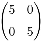
2×2 차 스칼라 행렬의 예

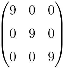
3×3 스칼라 행렬의 예

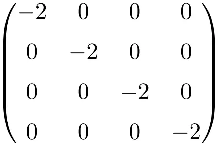
크기가 4×4인 스칼라 행렬의 예

스칼라 행렬의 속성

스칼라 행렬은 대각 행렬이기도 하므로 이 행렬 클래스의 많은 특성을 상속받는다는 것을 알 수 있습니다.

모든 스칼라 행렬은 대칭 행렬 이기도 합니다.

스칼라 행렬은 상부 삼각 행렬과 하부 삼각 행렬을 모두 포함합니다.

단위 행렬은 스칼라 행렬입니다.

모든 스칼라 행렬은 단위 행렬과 스칼라 수의 곱으로 얻을 수 있습니다.

$4 \cdot \begin{pmatrix} 1 & 0 & 0 \\[1.1ex] 0 & 1 & 0 \\[1.1ex] 0 & 0 & 1 \end{pmatrix} = \begin{pmatrix} 4 & 0 & 0 \\[1.1ex] 0 & 4 & 0 \\[1.1ex] 0 & 0 & 4 \end{pmatrix}$

제로 행렬은 스칼라 행렬이기도 합니다.

스칼라 행렬의 고유값(또는 고유값)은 주대각선의 요소입니다. 따라서 그들의 고유값은 항상 동일하며 행렬의 차원만큼 반복됩니다.

$\begin{pmatrix} 8 & 0 & 0 \\[1.1ex] 0 & 8 & 0 \\[1.1ex] 0 & 0 & 8 \end{pmatrix} \longrightarrow \ \lambda = 8 \ ; \ \lambda = 8 \ ; \ \lambda = 8$

스칼라 행렬의 수반은 또 다른 스칼라 행렬입니다. 또한 첨부된 행렬의 주대각선 값은 항상 행렬의 차수인 원래 행렬의 값인 1 입니다.

$\displaystyle A=\begin{pmatrix} 5 & 0 & 0 \\[1.1ex] 0 & 5 & 0 \\[1.1ex] 0 & 0 & 5 \end{pmatrix} \longrightarrow \text{Adj}(A)=\begin{pmatrix} 5^{3-1} & 0 & 0 \\[1.1ex] 0 & 5^{3-1} & 0 \\[1.1ex] 0 & 0 & 5^{3-1} \end{pmatrix}= \begin{pmatrix} 25 & 0 & 0 \\[1.1ex] 0 & 25 & 0 \\[1.1ex] 0 & 0 & 25 \end{pmatrix}$

스칼라 행렬을 사용한 연산

스칼라 행렬이 선형 대수학에서 널리 사용되는 이유 중 하나는 계산을 쉽게 수행할 수 있기 때문입니다. 이것이 수학에서 그것들이 그토록 중요한 이유이다.

이제 이러한 유형의 정사각 행렬을 사용하여 계산을 수행하는 것이 왜 그렇게 쉬운지 살펴보겠습니다.

스칼라 행렬의 덧셈과 뺄셈

두 개의 스칼라 행렬을 더하고 빼는 것은 매우 간단합니다. 주 대각선의 숫자를 더하거나 빼기만 하면 됩니다. 예를 들어:

$\displaystyle \begin{pmatrix} 4 & 0 & 0 \\[1.1ex] 0 & 4 & 0 \\[1.1ex] 0 & 0 & 4 \end{pmatrix} +\begin{pmatrix} 3 & 0 & 0 \\[1.1ex] 0 & 3 & 0 \\[1.1ex] 0 & 0 & 3 \end{pmatrix} = \begin{pmatrix} 7& 0 & 0 \\[1.1ex] 0 & 7 & 0 \\[1.1ex] 0 & 0 & 7 \end{pmatrix}$

스칼라 행렬 곱셈

덧셈과 뺄셈과 유사하게, 두 스칼라 행렬 간의 곱셈이나 행렬 곱을 풀려면 단순히 두 스칼라 행렬 사이의 대각선 요소를 곱하면 됩니다. 예를 들어:

$\displaystyle \begin{pmatrix} 2 & 0 & 0 \\[1.1ex] 0 & 2 & 0 \\[1.1ex] 0 & 0 & 2 \end{pmatrix} \cdot\begin{pmatrix} 6 & 0 & 0 \\[1.1ex] 0 & 6 & 0 \\[1.1ex] 0 & 0 & 6 \end{pmatrix} = \begin{pmatrix} 12 & 0 & 0 \\[1.1ex] 0 & 12 & 0 \\[1.1ex] 0 & 0 & 12 \end{pmatrix}$

스칼라 행렬의 힘

스칼라 행렬의 거듭제곱을 계산하는 것도 매우 간단합니다. 대각선의 각 요소를 지수로 올려야 합니다. 예를 들어:

 *** QuickLaTeX cannot compile formula:
\displaystyle\left. \begin{pmatrix} 2 & 0 & 0 \\[1.1ex] 0 & 2 & 0 \\[1.1ex] 0 & 0 & 2 \end{pmatrix}\right.^4=\begin{pmatrix} 2^ 4 & 0 & 0 \\[1.1ex] 0 & 2^

*** Error message:
Missing $ inserted.
leading text: \displaystyle
Missing { inserted.
leading text: \end{document}
\begin{pmatrix} on input line 9 ended by \end{document}.
leading text: \end{document}
Improper \prevdepth.
leading text: \end{document}
Missing $ inserted.
leading text: \end{document}
Missing } inserted.
leading text: \end{document}
Missing } inserted.
leading text: \end{document}
Missing \cr inserted.
leading text: \end{document}
Missing $ inserted.
leading text: \end{document}
You can't use `\end' in internal vertical mode.
leading text: \end{document}
\begin{pmatrix} on input line 9 ended by \end{document}.
leading text: \end{document}
Missing } inserted.
leading text: \end{document}
Missing \right. inserted.
leading text: \end{document}

& 0 \\[1.1ex] 0 & 0 & 2^4 \end{pmatrix}= \begin{pmatrix} 16 & 0 & 0 \\[1.1ex] 0 & 16 & 0 \\[1.1ex] 0 & 0 & 16 \end{pmatrix}

$<div class="adsb30" style=" margin:px; text-align:"></div> <h2 class="wp-block-heading"> Déterminant d’une matrice scalaire</h2> <p> Calculer le <strong>déterminant d’une matrice scalaire</strong> revient à résoudre le déterminant d’une matrice diagonale : le résultat est le produit des éléments sur la diagonale principale.” title=”Rendered by QuickLaTeX.com” height=”106″ width=”582″ style=”vertical-align: -4px;”></p> <p> \displaystyle \text{det}(A)= \prod_{i =1}^n a_i</p> <p class=$ $Regardez l'exercice résolu suivant dans lequel on trouve le déterminant d'une matrice scalaire en multipliant les éléments de sa diagonale principale :$

\displaystyle \begin{vmatrix} 7 & 0 & 0 \\[1.1ex] 0 & 7 & 0 \\[1.1ex] 0 & 0 & 7 \end{vmatrix} = 7 \cdot 7 \cdot 7 = \bm {343}

$En fait, puisque tous les éléments de la diagonale principale d'une matrice scalaire sont toujours égaux, pour trouver le résultat du déterminant, il suffit d'augmenter le numéro de la diagonale principale du nombre de fois qu'elle est répétée. Par conséquent, l'exercice précédent peut également être résolu de la manière suivante :$

\displaystyle \begin{vmatrix} 7 & 0 & 0 \\[1.1ex] 0 & 7 & 0 \\[1.1ex] 0 & 0 & 7 \end{vmatrix} = 7^3= \bm{343}

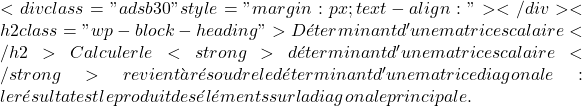
$Démontrer ce théorème est très simple : il suffit de calculer le déterminant d'une matrice scalaire par blocs (ou cofacteurs). Vous trouverez ci-dessous la <strong>démonstration</strong> de la formule utilisant une matrice scalaire générique :” title=”Rendered by QuickLaTeX.com” height=”62″ width=”1060″ style=”vertical-align: -4px;”></p> <p> \begin{aligned} \begin{vmatrix} a & 0 & 0 \\[1.1ex] 0 & a & 0 \\[1.1ex] 0 & 0 & a \end{vmatrix}& = a \cdot \begin{ vmatrix} a & 0 \\[1.1ex] 0 & a \end{vmatrix} – 0 \cdot \begin{vmatrix} 0 & 0 \\[1.1ex] 0 & a \end{vmatrix} + 0 \cdot \ 시작{vmatrix} 0 & a \\[1.1ex] 0 & 0 \end{vmatrix} \\[2ex] & =a \cdot (a\cdot a) – 0 \cdot 0 + 0 \cdot 0 \\[ 2ex] & = a \cdot a \cdot a \\[2ex] & = a^3 \end{aligned}</p> <p class=$ $Dans ce cas ça donne$

a^3

$car la matrice est d'ordre 3, mais il faut toujours l'élever à l'ordre de la matrice. <div class="adsb30" style=" margin:12px; text-align:center"> <div id="ezoic-pub-ad-placeholder-118"></div> </div> <h2 class="wp-block-heading"> Inverser une matrice scalaire</h2> <p> Une matrice scalaire <strong>est inversible si, et seulement si, tous les éléments de la diagonale principale sont différents de 0</strong> . Dans ce cas on dit que la matrice scalaire est une matrice régulière. De plus, l’inverse d’une matrice scalaire sera toujours une autre matrice scalaire avec les <strong>inverses</strong> de la diagonale principale :” title=”Rendered by QuickLaTeX.com” height=”174″ width=”1250″ style=”vertical-align: -5px;”></p> <p> \displaystyle A= \begin{pmatrix} 9 & 0 & 0 \\[1.1ex] 0 & 9 & 0 \\[1.1ex] 0 & 0 & 9 \end{pmatrix} \ \longrightarrow \ A^{-1 }=\begin{pmatrix} \frac{1}{9} & 0 & 0 \\[1.1ex] 0 & \frac{1}{9} & 0 \\[1.1ex] 0 & 0 & \frac{ 1}{9} \end{pmatrix}</p> <p class=$ $D'autre part, de la caractéristique précédente, on peut déduire que le déterminant d'une matrice scalaire inversée est le résultat de la multiplication des inverses de la diagonale principale :$

\displaystyle B= \begin{pmatrix} 2 & 0 & 0 \\[1.1ex] 0 & 2 & 0 \\[1.1ex] 0 & 0 & 2 \end{pmatrix} \displaystyle\left| B^{-1}\right|=\cfrac{1}{2} \cdot \cfrac{1}{2} \cdot \cfrac{1}{2}=\cfrac{1}{8} = $0.125