スカラー行列 - マソリティ

このページでは、スカラー行列とは何か、およびスカラー行列を完全に理解できるようにいくつかのスカラー行列の例を示します。さらに、スカラー行列のすべてのプロパティと、スカラー行列を操作する利点を確認できるようになります。最後に、スカラー行列の行列式を計算する方法と、このタイプの行列を反転する方法について説明します。

スカラー行列とは何ですか?

スカラー行列は、主対角上のすべての値が等しい対角行列です。

これはスカラー行列の定義ですが、例を見るとよりよく理解できると思います。 😉

スカラー配列の例

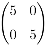
次数 2×2 のスカラー行列の例

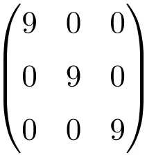
3×3 スカラー行列の例

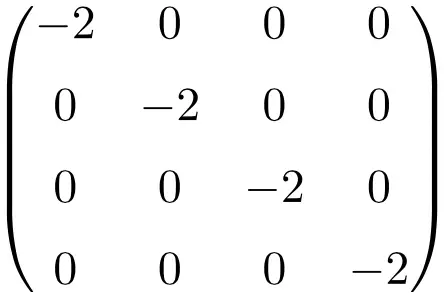
サイズ 4×4 のスカラー行列の例

スカラー行列のプロパティ

スカラー行列は対角行列でもあるため、この行列クラスの多くの特性を継承していることがわかります。

すべてのスカラー行列も対称行列です。

スカラー行列は、上三角行列と下三角行列の両方です。

単位行列はスカラー行列です。

任意のスカラー行列は単位行列とスカラー数の積から取得できます。

$4 \cdot \begin{pmatrix} 1 & 0 & 0 \\[1.1ex] 0 & 1 & 0 \\[1.1ex] 0 & 0 & 1 \end{pmatrix} = \begin{pmatrix} 4 & 0 & 0 \\[1.1ex] 0 & 4 & 0 \\[1.1ex] 0 & 0 & 4 \end{pmatrix}$

ゼロ行列もスカラー行列です。

スカラー行列の固有値 (または固有値) は、その主対角要素です。したがって、それらの固有値は常に同じになり、行列の次元と同じ回数繰り返されます。

$\begin{pmatrix} 8 & 0 & 0 \\[1.1ex] 0 & 8 & 0 \\[1.1ex] 0 & 0 & 8 \end{pmatrix} \longrightarrow \ \lambda = 8 \ ; \ \lambda = 8 \ ; \ \lambda = 8$

スカラー行列の随伴物は別のスカラー行列です。さらに、アタッチされた行列の主対角の値は、常に元の行列の行列の次数 – 1 に引き上げられたものになります。

$\displaystyle A=\begin{pmatrix} 5 & 0 & 0 \\[1.1ex] 0 & 5 & 0 \\[1.1ex] 0 & 0 & 5 \end{pmatrix} \longrightarrow \text{Adj}(A)=\begin{pmatrix} 5^{3-1} & 0 & 0 \\[1.1ex] 0 & 5^{3-1} & 0 \\[1.1ex] 0 & 0 & 5^{3-1} \end{pmatrix}= \begin{pmatrix} 25 & 0 & 0 \\[1.1ex] 0 & 25 & 0 \\[1.1ex] 0 & 0 & 25 \end{pmatrix}$

スカラー行列を使用した演算

スカラー行列が線形代数で非常に広く使用されている理由の 1 つは、計算の実行が容易であることです。これが、数学においてそれらが非常に重要である理由です。

それでは、このタイプの正方行列を使用して計算を行うのがなぜ非常に簡単なのかを見てみましょう。

スカラー行列の加算と減算

2 つのスカラー行列の加算 (および減算) は非常に簡単です。主な対角線上の数値を加算 (または減算) するだけです。例えば：

$\displaystyle \begin{pmatrix} 4 & 0 & 0 \\[1.1ex] 0 & 4 & 0 \\[1.1ex] 0 & 0 & 4 \end{pmatrix} +\begin{pmatrix} 3 & 0 & 0 \\[1.1ex] 0 & 3 & 0 \\[1.1ex] 0 & 0 & 3 \end{pmatrix} = \begin{pmatrix} 7& 0 & 0 \\[1.1ex] 0 & 7 & 0 \\[1.1ex] 0 & 0 & 7 \end{pmatrix}$

スカラー行列の乗算

加算と減算と同様に、2 つのスカラー行列間の乗算または行列積を解くには、単純にそれらの間の対角要素を乗算します。例えば：

$\displaystyle \begin{pmatrix} 2 & 0 & 0 \\[1.1ex] 0 & 2 & 0 \\[1.1ex] 0 & 0 & 2 \end{pmatrix} \cdot\begin{pmatrix} 6 & 0 & 0 \\[1.1ex] 0 & 6 & 0 \\[1.1ex] 0 & 0 & 6 \end{pmatrix} = \begin{pmatrix} 12 & 0 & 0 \\[1.1ex] 0 & 12 & 0 \\[1.1ex] 0 & 0 & 12 \end{pmatrix}$

スカラー行列の力

スカラー行列の累乗の計算も非常に簡単です。対角の各要素を指数化する必要があります。例えば：

 *** QuickLaTeX cannot compile formula:
\displaystyle\left. \begin{pmatrix} 2 & 0 & 0 \\[1.1ex] 0 & 2 & 0 \\[1.1ex] 0 & 0 & 2 \end{pmatrix}\right.^4=\begin{pmatrix} 2^ 4 & 0 & 0 \\[1.1ex] 0 & 2^

*** Error message:
Missing $ inserted.
leading text: \displaystyle
Missing { inserted.
leading text: \end{document}
\begin{pmatrix} on input line 9 ended by \end{document}.
leading text: \end{document}
Improper \prevdepth.
leading text: \end{document}
Missing $ inserted.
leading text: \end{document}
Missing } inserted.
leading text: \end{document}
Missing } inserted.
leading text: \end{document}
Missing \cr inserted.
leading text: \end{document}
Missing $ inserted.
leading text: \end{document}
You can't use `\end' in internal vertical mode.
leading text: \end{document}
\begin{pmatrix} on input line 9 ended by \end{document}.
leading text: \end{document}
Missing } inserted.
leading text: \end{document}
Missing \right. inserted.
leading text: \end{document}

& 0 \\[1.1ex] 0 & 0 & 2^4 \end{pmatrix}= \begin{pmatrix} 16 & 0 & 0 \\[1.1ex] 0 & 16 & 0 \\[1.1ex] 0 & 0 & 16 \end{pmatrix}

$<div class="adsb30" style=" margin:px; text-align:"></div> <h2 class="wp-block-heading"> Déterminant d’une matrice scalaire</h2> <p> Calculer le <strong>déterminant d’une matrice scalaire</strong> revient à résoudre le déterminant d’une matrice diagonale : le résultat est le produit des éléments sur la diagonale principale.” title=”Rendered by QuickLaTeX.com” height=”106″ width=”582″ style=”vertical-align: -4px;”></p> <p> \displaystyle \text{det}(A)= \prod_{i =1}^n a_i</p> <p class=$ $Regardez l'exercice résolu suivant dans lequel on trouve le déterminant d'une matrice scalaire en multipliant les éléments de sa diagonale principale :$

\displaystyle \begin{vmatrix} 7 & 0 & 0 \\[1.1ex] 0 & 7 & 0 \\[1.1ex] 0 & 0 & 7 \end{vmatrix} = 7 \cdot 7 \cdot 7 = \bm {343}

$En fait, puisque tous les éléments de la diagonale principale d'une matrice scalaire sont toujours égaux, pour trouver le résultat du déterminant, il suffit d'augmenter le numéro de la diagonale principale du nombre de fois qu'elle est répétée. Par conséquent, l'exercice précédent peut également être résolu de la manière suivante :$

\displaystyle \begin{vmatrix} 7 & 0 & 0 \\[1.1ex] 0 & 7 & 0 \\[1.1ex] 0 & 0 & 7 \end{vmatrix} = 7^3= \bm{343}

$Démontrer ce théorème est très simple : il suffit de calculer le déterminant d'une matrice scalaire par blocs (ou cofacteurs). Vous trouverez ci-dessous la <strong>démonstration</strong> de la formule utilisant une matrice scalaire générique :” title=”Rendered by QuickLaTeX.com” height=”62″ width=”1060″ style=”vertical-align: -4px;”></p> <p> \begin{aligned} \begin{vmatrix} a & 0 & 0 \\[1.1ex] 0 & a & 0 \\[1.1ex] 0 & 0 & a \end{vmatrix}& = a \cdot \begin{ vmatrix} a & 0 \\[1.1ex] 0 & a \end{vmatrix} – 0 \cdot \begin{vmatrix} 0 & 0 \\[1.1ex] 0 & a \end{vmatrix} + 0 \cdot \ begin{vmatrix} 0 & a \\[1.1ex] 0 & 0 \end{vmatrix} \\[2ex] & =a \cdot (a\cdot a) – 0 \cdot 0 + 0 \cdot 0 \\[ 2ex] & = a \cdot a \cdot a \\[2ex] & = a^3 \end{aligned}</p> <p class=$ $Dans ce cas ça donne$

a^3

$car la matrice est d'ordre 3, mais il faut toujours l'élever à l'ordre de la matrice. <div class="adsb30" style=" margin:12px; text-align:center"> <div id="ezoic-pub-ad-placeholder-118"></div> </div> <h2 class="wp-block-heading"> Inverser une matrice scalaire</h2> <p> Une matrice scalaire <strong>est inversible si, et seulement si, tous les éléments de la diagonale principale sont différents de 0</strong> . Dans ce cas on dit que la matrice scalaire est une matrice régulière. De plus, l’inverse d’une matrice scalaire sera toujours une autre matrice scalaire avec les <strong>inverses</strong> de la diagonale principale :” title=”Rendered by QuickLaTeX.com” height=”174″ width=”1250″ style=”vertical-align: -5px;”></p> <p> \displaystyle A= \begin{pmatrix} 9 & 0 & 0 \\[1.1ex] 0 & 9 & 0 \\[1.1ex] 0 & 0 & 9 \end{pmatrix} \ \longrightarrow \ A^{-1 }=\begin{pmatrix} \frac{1}{9} & 0 & 0 \\[1.1ex] 0 & \frac{1}{9} & 0 \\[1.1ex] 0 & 0 & \frac{ 1}{9} \end{p行列}</p> <p class=$ $D'autre part, de la caractéristique précédente, on peut déduire que le déterminant d'une matrice scalaire inversée est le résultat de la multiplication des inverses de la diagonale principale :$

\displaystyle B= \begin{pmatrix} 2 & 0 & 0 \\[1.1ex] 0 & 2 & 0 \\[1.1ex] 0 & 0 & 2 \end{pmatrix} \displaystyle\left| B^{-1}\right|=\cfrac{1}{2} \cdot \cfrac{1}{2} \cdot \cfrac{1}{2}=\cfrac{1}{8} = $0.125