Auf dieser Seite finden Sie, was eine Skalarmatrix ist, und einige Beispiele für Skalarmatrizen, damit es perfekt verstanden wird. Darüber hinaus können Sie alle Eigenschaften von Skalarmatrizen und die Vorteile der Durchführung von Operationen mit ihnen erkennen. Abschließend erklären wir, wie man die Determinante einer Skalarmatrix berechnet und wie man diese Art von Matrix invertiert.
Was ist eine Skalarmatrix?
Eine Skalarmatrix ist eine Diagonalmatrix , bei der alle Werte auf der Hauptdiagonale gleich sind.
Dies ist die Definition einer Skalarmatrix, aber ich bin sicher, dass man sie anhand von Beispielen besser verstehen kann: 😉
Beispiele für Skalar-Arrays
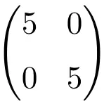
Beispiel einer Skalarmatrix der Ordnung 2×2
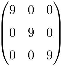
Beispiel einer 3×3-Skalarmatrix
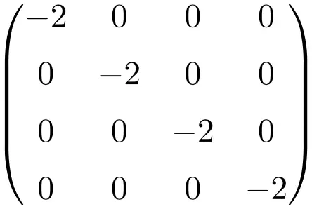
Beispiel einer Skalarmatrix der Größe 4×4
Eigenschaften von Skalarmatrizen
Die Skalarmatrix ist auch eine Diagonalmatrix, Sie werden also sehen, dass sie viele Merkmale dieser Matrixklasse erbt:
- Alle Skalarmatrizen sind auch symmetrische Matrizen .
- Eine Skalarmatrix ist sowohl eine obere Dreiecksmatrix als auch eine untere Dreiecksmatrix .
- Die Identitätsmatrix ist eine Skalarmatrix.
- Jede Skalarmatrix kann aus dem Produkt einer Identitätsmatrix und einer Skalarzahl erhalten werden.
![4 \cdot \begin{pmatrix} 1 & 0 & 0 \\[1.1ex] 0 & 1 & 0 \\[1.1ex] 0 & 0 & 1 \end{pmatrix} = \begin{pmatrix} 4 & 0 & 0 \\[1.1ex] 0 & 4 & 0 \\[1.1ex] 0 & 0 & 4 \end{pmatrix}](https://mathority.org/wp-content/ql-cache/quicklatex.com-b77f7d177c2769b0847de258adfd1386_l3.png "Rendered by QuickLaTeX.com")
- Die Nullmatrix ist ebenfalls eine Skalarmatrix.
- Die Eigenwerte (oder Eigenwerte) einer Skalarmatrix sind die Elemente ihrer Hauptdiagonale. Daher sind ihre Eigenwerte immer gleich und werden so oft wiederholt, wie die Dimension der Matrix.
![\begin{pmatrix} 8 & 0 & 0 \\[1.1ex] 0 & 8 & 0 \\[1.1ex] 0 & 0 & 8 \end{pmatrix} \longrightarrow \ \lambda = 8 \ ; \ \lambda = 8 \ ; \ \lambda = 8](https://mathority.org/wp-content/ql-cache/quicklatex.com-2513b8d4aeb6d932d9870934102a1637_l3.png "Rendered by QuickLaTeX.com")
- Der Adjungierte einer Skalarmatrix ist eine andere Skalarmatrix. Darüber hinaus sind die Werte der Hauptdiagonalen der angehängten Matrix immer diejenigen der ursprünglichen Matrix, erhöht auf die Matrixordnung – 1 .
![\displaystyle A=\begin{pmatrix} 5 & 0 & 0 \\[1.1ex] 0 & 5 & 0 \\[1.1ex] 0 & 0 & 5 \end{pmatrix} \longrightarrow \text{Adj}(A)=\begin{pmatrix} 5^{3-1} & 0 & 0 \\[1.1ex] 0 & 5^{3-1} & 0 \\[1.1ex] 0 & 0 & 5^{3-1} \end{pmatrix}= \begin{pmatrix} 25 & 0 & 0 \\[1.1ex] 0 & 25 & 0 \\[1.1ex] 0 & 0 & 25 \end{pmatrix}](https://mathority.org/wp-content/ql-cache/quicklatex.com-1f7e94cc5a528abace04016dc263c8f9_l3.png "Rendered by QuickLaTeX.com")
Operationen mit Skalarmatrizen
Einer der Gründe, warum Skalarmatrizen in der linearen Algebra so häufig verwendet werden, ist die einfache Durchführung von Berechnungen. Deshalb sind sie in der Mathematik so wichtig.
Sehen wir uns also an, warum es so einfach ist, Berechnungen mit dieser Art von quadratischer Matrix durchzuführen:
Addition und Subtraktion von Skalarmatrizen
Das Addieren (und Subtrahieren) zweier Skalarmatrizen ist sehr einfach: Addieren (oder subtrahieren) Sie einfach die Zahlen auf den Hauptdiagonalen. Zum Beispiel:
![\displaystyle \begin{pmatrix} 4 & 0 & 0 \\[1.1ex] 0 & 4 & 0 \\[1.1ex] 0 & 0 & 4 \end{pmatrix} +\begin{pmatrix} 3 & 0 & 0 \\[1.1ex] 0 & 3 & 0 \\[1.1ex] 0 & 0 & 3 \end{pmatrix} = \begin{pmatrix} 7& 0 & 0 \\[1.1ex] 0 & 7 & 0 \\[1.1ex] 0 & 0 & 7 \end{pmatrix}](https://mathority.org/wp-content/ql-cache/quicklatex.com-761de4b4c9bdbbc835b366b21d8cfc2d_l3.png "Rendered by QuickLaTeX.com")
Skalarmatrixmultiplikation
Um eine Multiplikation oder ein Matrixprodukt zwischen zwei Skalarmatrizen zu lösen, multiplizieren Sie ähnlich wie bei der Addition und Subtraktion einfach die Elemente der Diagonalen zwischen ihnen. Zum Beispiel:
![\displaystyle \begin{pmatrix} 2 & 0 & 0 \\[1.1ex] 0 & 2 & 0 \\[1.1ex] 0 & 0 & 2 \end{pmatrix} \cdot\begin{pmatrix} 6 & 0 & 0 \\[1.1ex] 0 & 6 & 0 \\[1.1ex] 0 & 0 & 6 \end{pmatrix} = \begin{pmatrix} 12 & 0 & 0 \\[1.1ex] 0 & 12 & 0 \\[1.1ex] 0 & 0 & 12 \end{pmatrix}](https://mathority.org/wp-content/ql-cache/quicklatex.com-d30acbf9c6ad31625f8253549e659b02_l3.png "Rendered by QuickLaTeX.com")
Leistung skalarer Matrizen
Auch die Berechnung der Potenz einer Skalarmatrix ist sehr einfach: Man muss jedes Element der Diagonale auf den Exponenten erhöhen. Zum Beispiel:
 *** QuickLaTeX cannot compile formula:
\displaystyle\left. \begin{pmatrix} 2 & 0 & 0 \\[1.1ex] 0 & 2 & 0 \\[1.1ex] 0 & 0 & 2 \end{pmatrix}\right.^4=\begin{pmatrix} 2^ 4 & 0 & 0 \\[1.1ex] 0 & 2^

*** Error message:
Missing $ inserted.
leading text: \displaystyle
Missing { inserted.
leading text: \end{document}
\begin{pmatrix} on input line 9 ended by \end{document}.
leading text: \end{document}
Improper \prevdepth.
leading text: \end{document}
Missing $ inserted.
leading text: \end{document}
Missing } inserted.
leading text: \end{document}
Missing } inserted.
leading text: \end{document}
Missing \cr inserted.
leading text: \end{document}
Missing $ inserted.
leading text: \end{document}
You can't use `\end' in internal vertical mode.
leading text: \end{document}
\begin{pmatrix} on input line 9 ended by \end{document}.
leading text: \end{document}
Missing } inserted.
leading text: \end{document}
Missing \right. inserted.
leading text: \end{document}
& 0 \\[1.1ex] 0 & 0 & 2^4 \end{pmatrix}= \begin{pmatrix} 16 & 0 & 0 \\[1.1ex] 0 & 16 & 0 \\[1.1ex] 0 & 0 & 16 \end{pmatrix}

\displaystyle \begin{vmatrix} 7 & 0 & 0 \\[1.1ex] 0 & 7 & 0 \\[1.1ex] 0 & 0 & 7 \end{vmatrix} = 7 \cdot 7 \cdot 7 = \bm {343}

\displaystyle \begin{vmatrix} 7 & 0 & 0 \\[1.1ex] 0 & 7 & 0 \\[1.1ex] 0 & 0 & 7 \end{vmatrix} = 7^3= \bm{343}
![Démontrer ce théorème est très simple : il suffit de calculer le déterminant d'une matrice scalaire par blocs (ou cofacteurs). Vous trouverez ci-dessous la <strong>démonstration</strong> de la formule utilisant une matrice scalaire générique :“ title=“Rendered by QuickLaTeX.com“ height=“62″ width=“1060″ style=“vertical-align: -4px;“></p>
<p> \begin{aligned} \begin{vmatrix} a & 0 & 0 \\[1.1ex] 0 & a & 0 \\[1.1ex] 0 & 0 & a \end{vmatrix}& = a \cdot \begin{ vmatrix} a & 0 \\[1.1ex] 0 & a \end{vmatrix} – 0 \cdot \begin{vmatrix} 0 & 0 \\[1.1ex] 0 & a \end{vmatrix} + 0 \cdot \ begin{vmatrix} 0 & a \\[1.1ex] 0 & 0 \end{vmatrix} \\[2ex] & =a \cdot (a\cdot a) – 0 \cdot 0 + 0 \cdot 0 \\[ 2ex] & = a \cdot a \cdot a \\[2ex] & = a^3 \end{aligned}</p>
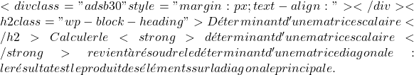
<p class=](https://mathority.org/wp-content/ql-cache/quicklatex.com-d24f9aa91fc9fe8ed74f705f83be3b32_l3.png)

a^3
![car la matrice est d'ordre 3, mais il faut toujours l'élever à l'ordre de la matrice.
<div class="adsb30" style=" margin:12px; text-align:center">
<div id="ezoic-pub-ad-placeholder-118"></div>
</div>
<h2 class="wp-block-heading"> Inverser une matrice scalaire</h2>
<p> Une matrice scalaire <strong>est inversible si, et seulement si, tous les éléments de la diagonale principale sont différents de 0</strong> . Dans ce cas on dit que la matrice scalaire est une matrice régulière. De plus, l’inverse d’une matrice scalaire sera toujours une autre matrice scalaire avec les <strong>inverses</strong> de la diagonale principale :“ title=“Rendered by QuickLaTeX.com“ height=“174″ width=“1250″ style=“vertical-align: -5px;“></p>
<p> \displaystyle A= \begin{pmatrix} 9 & 0 & 0 \\[1.1ex] 0 & 9 & 0 \\[1.1ex] 0 & 0 & 9 \end{pmatrix} \ \longrightarrow \ A^{-1 }=\begin{pmatrix} \frac{1}{9} & 0 & 0 \\[1.1ex] 0 & \frac{1}{9} & 0 \\[1.1ex] 0 & 0 & \frac{ 1}{9} \end{pmatrix}</p>
<p class=](https://mathority.org/wp-content/ql-cache/quicklatex.com-49f5afdd3e1e9918f5323139662a2138_l3.png)

\displaystyle B= \begin{pmatrix} 2 & 0 & 0 \\[1.1ex] 0 & 2 & 0 \\[1.1ex] 0 & 0 & 2 \end{pmatrix} \displaystyle\left| B^{-1}\right|=\cfrac{1}{2} \cdot \cfrac{1}{2} \cdot \cfrac{1}{2}=\cfrac{1}{8} = $0,125