在本页中,我们将了解如何计算矩阵的幂。您还将找到矩阵幂的示例和逐步解决的练习,这将帮助您完全理解它。您还将了解什么是矩阵的 n 次方以及如何求它。
矩阵的幂是如何计算的?
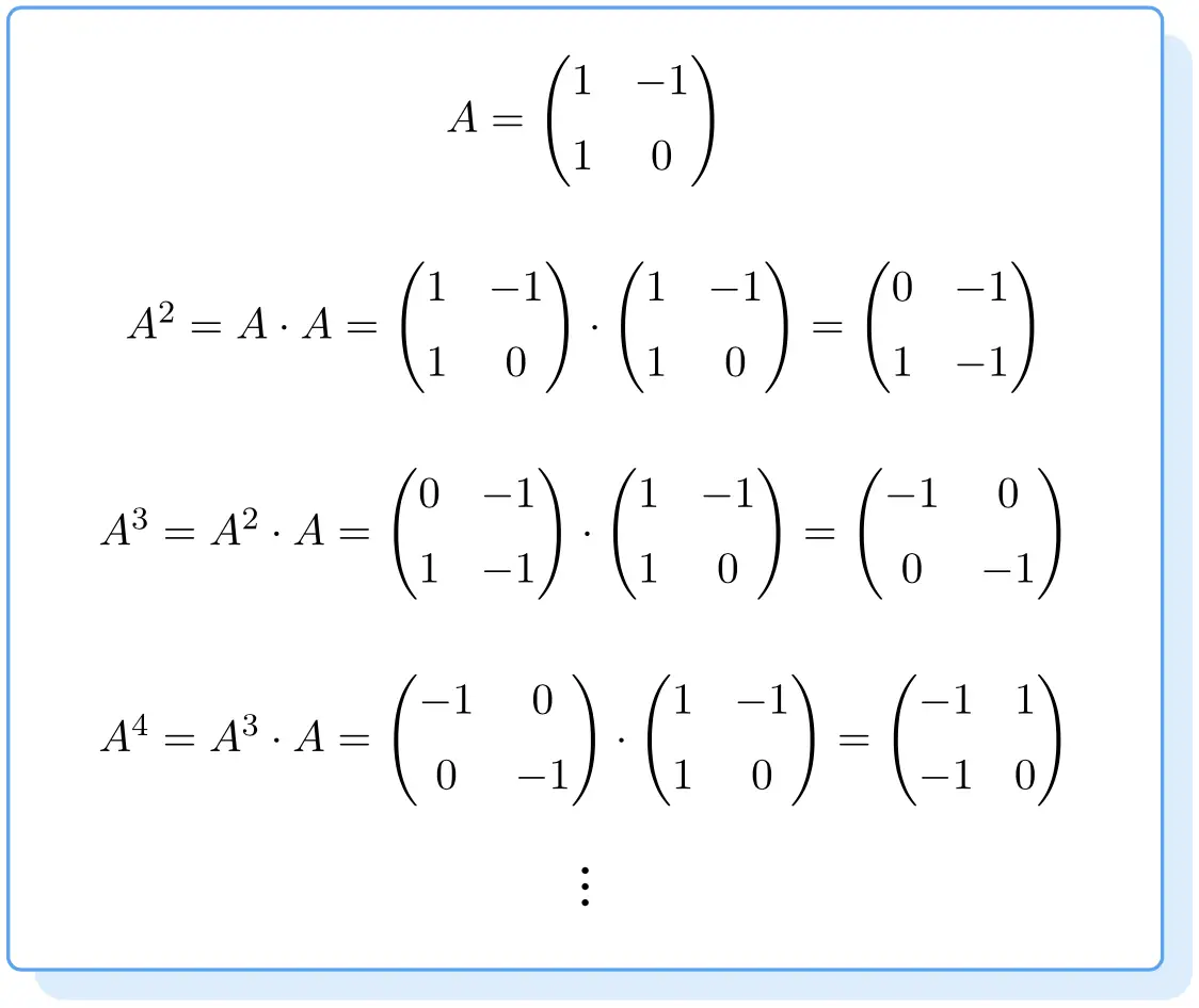
要计算矩阵 的幂,您必须将矩阵与其自身相乘,次数与指数所示的次数相同。例如:

因此,要获得矩阵的幂,您需要知道如何解决矩阵乘法。否则你无法计算功率矩阵。
计算矩阵幂的示例:
因此,方阵的幂是通过矩阵乘以自身来计算的。类似地,立方矩阵等于矩阵本身的平方矩阵。类似地,要求矩阵四次方的幂,必须将矩阵三次方乘以矩阵本身。等等。
您应该知道矩阵幂的一个重要属性:只有当矩阵为方阵时(即行数与列数相同时)才能计算矩阵的幂。
矩阵的n次方是多少?
矩阵的n次方是一个表达式,可以让我们轻松计算矩阵的任意次方。
矩阵的幂通常遵循某种模式。因此,如果我们能够破译它们遵循的序列,我们将能够计算任何幂,而不必进行所有乘法。
这意味着我们可以找到一个公式来计算矩阵的 n 次方,而无需计算所有次方。
发现权力所遵循的模式的提示:
- 指数的奇偶性。偶次幂可能是一种方式,奇次幂是另一种方式。
- 标志的变化。例如,偶数次方的元素可能为正,而奇数次方的元素可能为负,或者反之亦然。
- 重复:同一矩阵是否每隔一定次数的幂重复一次。
- 我们还必须看看指数和矩阵元素之间是否存在关系。
计算矩阵 n 次方的示例:
- 是

下面的矩阵,计算

和

。
![\displaystyle A = \begin{pmatrix} 1 & 1 \\[1.1ex] 1 & 1 \end{pmatrix}](https://mathority.org/wp-content/ql-cache/quicklatex.com-60016ce1c6799c93007526681fbf4894_l3.png "Rendered by QuickLaTeX.com")
我们首先计算矩阵的几次幂
,尝试猜测幂所遵循的模式。所以我们计算

,

,

和

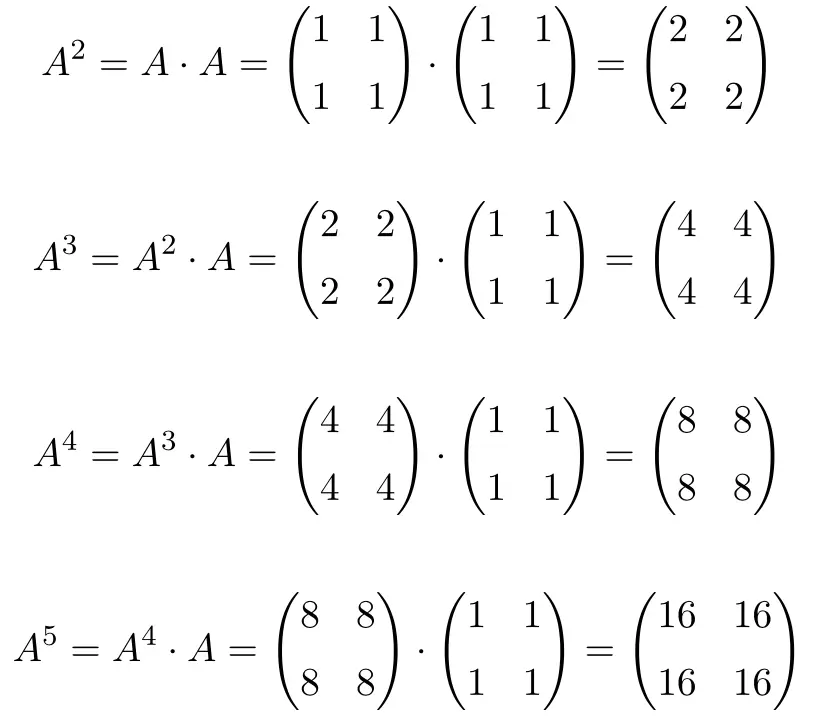
当计算至

,我们看到矩阵的幂
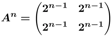
它们遵循一个模式:每次幂增加,结果都会乘以 2。因此,所有矩阵都是 2 的幂:
![\displaystyle A^2= \begin{pmatrix} 2 & 2 \\[1.1ex] 2 & 2 \end{pmatrix} =\begin{pmatrix} 2^1 & 2^1 \\[1.1ex] 2^1 & 2^1 \end{pmatrix}](https://mathority.org/wp-content/ql-cache/quicklatex.com-4ec7ee835cf9eda6a4f9d497e8baff79_l3.png "Rendered by QuickLaTeX.com")
![\displaystyle A^3= \begin{pmatrix} 4 & 4 \\[1.1ex] 4 & 4 \end{pmatrix}=\begin{pmatrix} 2^2 & 2^2 \\[1.1ex] 2^2 & 2^2 \end{pmatrix}](https://mathority.org/wp-content/ql-cache/quicklatex.com-69c6ff0f4de92192584dadc4719167c7_l3.png "Rendered by QuickLaTeX.com")
![\displaystyle A^4= \begin{pmatrix} 8 & 8 \\[1.1ex] 8 & 8 \end{pmatrix}=\begin{pmatrix} 2^3 & 2^3 \\[1.1ex] 2^3 & 2^3 \end{pmatrix}](https://mathority.org/wp-content/ql-cache/quicklatex.com-f724a50b220b3026d53e40ee17870359_l3.png "Rendered by QuickLaTeX.com")
![\displaystyle A^5= \begin{pmatrix} 16 & 16 \\[1.1ex] 16 & 16 \end{pmatrix}=\begin{pmatrix} 2^4 & 2^4 \\[1.1ex] 2^4 & 2^4 \end{pmatrix}](https://mathority.org/wp-content/ql-cache/quicklatex.com-f5f08f7cc00465a6a098ce7d752aa66f_l3.png "Rendered by QuickLaTeX.com")
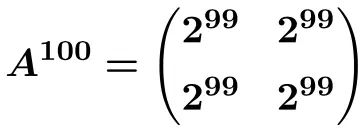
因此我们可以推导出矩阵n次方的公式

从这个公式我们可以计算出

解决了矩阵功率问题
练习1
考虑以下维度为 2×2 的矩阵:
![\displaystyle A=\begin{pmatrix} 1 & 2 \\[1.1ex] -1 & 1 \end{pmatrix}](https://mathority.org/wp-content/ql-cache/quicklatex.com-cdf81cf9fb956a144c7bda96a84ec7db_l3.png "Rendered by QuickLaTeX.com")
计算:

要计算矩阵的幂,必须将矩阵一乘一。因此,我们首先计算

![\displaystyle A^2= A \cdot A = \begin{pmatrix} 1 & 2 \\[1.1ex] -1 & 1 \end{pmatrix} \cdot \begin{pmatrix} 1 & 2 \\[1.1ex] -1 & 1 \end{pmatrix} = \begin{pmatrix} -1 & 4 \\[1.1ex] -2 & -1\end{pmatrix}](https://mathority.org/wp-content/ql-cache/quicklatex.com-24916b0b0e4431b0a2ee2b09875dc903_l3.png "Rendered by QuickLaTeX.com")
现在我们计算

![\displaystyle A^3= A^2 \cdot A = \begin{pmatrix} -1 & 4 \\[1.1ex] -2 & -1 \end{pmatrix} \cdot \begin{pmatrix} 1 & 2 \\[1.1ex] -1 & 1 \end{pmatrix} =\begin{pmatrix} -5 & 2 \\[1.1ex] -1 & -5 \end{pmatrix}](https://mathority.org/wp-content/ql-cache/quicklatex.com-57f79bd420c0044c84a64b431035b8ea_l3.png "Rendered by QuickLaTeX.com")
最后我们计算

![\displaystyle A^4= A^3 \cdot A = \begin{pmatrix} -5 & 2 \\[1.1ex] -1 & -5 \end{pmatrix} \cdot \begin{pmatrix} 1 & 2 \\[1.1ex] -1 & 1 \end{pmatrix} = \begin{pmatrix} \bm{-7} & \bm{-8} \\[1.1ex] \bm{4} & \bm{-7} \end{pmatrix}](https://mathority.org/wp-content/ql-cache/quicklatex.com-bbc2ad8229ee141b323c9bbcc9df00fd_l3.png "Rendered by QuickLaTeX.com")
练习2
考虑以下 2 阶矩阵:
![\displaystyle A=\begin{pmatrix} 1 & 0 \\[1.1ex] 0 & 3 \end{pmatrix}](https://mathority.org/wp-content/ql-cache/quicklatex.com-33db03560b5c28f45eef9aa293484603_l3.png "Rendered by QuickLaTeX.com")
计算:

的幂太大而无法手动计算,因此矩阵幂必须遵循某种模式。那么我们来计算一下

尝试理解它们遵循的顺序:
![\displaystyle A^2= A \cdot A = \begin{pmatrix} 1 & 0 \\[1.1ex] 0 & 3 \end{pmatrix} \cdot \begin{pmatrix}1 & 0 \\[1.1ex] 0 & 3 \end{pmatrix} = \begin{pmatrix} 1 & 0 \\[1.1ex] 0 & 9 \end{pmatrix}](https://mathority.org/wp-content/ql-cache/quicklatex.com-cb9646cc984d754d2a618e6223e93cd3_l3.png "Rendered by QuickLaTeX.com")
![\displaystyle A^3= A^2 \cdot A = \begin{pmatrix} 1 & 0 \\[1.1ex] 0 & 9 \end{pmatrix} \cdot \begin{pmatrix}1 & 0 \\[1.1ex] 0 & 3 \end{pmatrix} = \begin{pmatrix} 1 & 0 \\[1.1ex] 0 & 27 \end{pmatrix}](https://mathority.org/wp-content/ql-cache/quicklatex.com-22fdee28399b9115de98a214ba0c8473_l3.png "Rendered by QuickLaTeX.com")
![\displaystyle A^4= A^3 \cdot A = \begin{pmatrix}1 & 0 \\[1.1ex] 0 & 27 \end{pmatrix} \cdot \begin{pmatrix}1 & 0 \\[1.1ex] 0 & 3 \end{pmatrix} = \begin{pmatrix} 1 & 0 \\[1.1ex] 0 & 81 \end{pmatrix}](https://mathority.org/wp-content/ql-cache/quicklatex.com-1a085a2338ce1e74885ca04bbd0011a7_l3.png "Rendered by QuickLaTeX.com")
![\displaystyle A^5= A^4 \cdot A = \begin{pmatrix}1 & 0 \\[1.1ex] 0 & 81 \end{pmatrix} \cdot \begin{pmatrix}1 & 0 \\[1.1ex] 0 & 3 \end{pmatrix} = \begin{pmatrix} 1 & 0 \\[1.1ex] 0 & 243 \end{pmatrix}](https://mathority.org/wp-content/ql-cache/quicklatex.com-3dc357146829da8323a0755fa16a8ca8_l3.png "Rendered by QuickLaTeX.com")
这样我们就可以看到幂遵循的模式:在每个幂上,除了第二行第二列中的元素乘以 3 之外,所有数字都保持相同。因此,所有数字始终保持相同。最后一个元素是 3 的幂:
![\displaystyle A=\begin{pmatrix} 1 & 0 \\[1.1ex] 0 & 3 \end{pmatrix}=\begin{pmatrix} 1 & 0 \\[1.1ex] 0 & 3^1 \end{pmatrix}](https://mathority.org/wp-content/ql-cache/quicklatex.com-a0bfa34768808832e0fd5d3f730eb27b_l3.png "Rendered by QuickLaTeX.com")
![\displaystyle A^2=\begin{pmatrix} 1 & 0 \\[1.1ex] 0 & 9 \end{pmatrix}=\begin{pmatrix} 1 & 0 \\[1.1ex] 0 & 3^2 \end{pmatrix}](https://mathority.org/wp-content/ql-cache/quicklatex.com-f6e007f5ad5d38fd887d39f00bd2b9fc_l3.png "Rendered by QuickLaTeX.com")
![\displaystyle A^3=\begin{pmatrix} 1 & 0 \\[1.1ex] 0 & 27 \end{pmatrix}=\begin{pmatrix} 1 & 0 \\[1.1ex] 0 & 3^3 \end{pmatrix}](https://mathority.org/wp-content/ql-cache/quicklatex.com-585d8a00f418b50f60b4f95d87c5839c_l3.png "Rendered by QuickLaTeX.com")
![\displaystyle A^4=\begin{pmatrix} 1 & 0 \\[1.1ex] 0 & 81 \end{pmatrix}=\begin{pmatrix} 1 & 0 \\[1.1ex] 0 & 3^4 \end{pmatrix}](https://mathority.org/wp-content/ql-cache/quicklatex.com-dec6b9db4b59d9759adf85cee442cca3_l3.png "Rendered by QuickLaTeX.com")
![\displaystyle A^5=\begin{pmatrix} 1 & 0 \\[1.1ex] 0 & 243 \end{pmatrix}=\begin{pmatrix} 1 & 0 \\[1.1ex] 0 & 3^5 \end{pmatrix}](https://mathority.org/wp-content/ql-cache/quicklatex.com-f7244b46950df4d9107cbdb7ad004e17_l3.png "Rendered by QuickLaTeX.com")
所以矩阵的n次方公式

东方:
![\displaystyle A^n=\begin{pmatrix} 1 & 0 \\[1.1ex] 0 & 3^n\end{pmatrix}](https://mathority.org/wp-content/ql-cache/quicklatex.com-beec2f1ed3e47902de0f25fe1901e294_l3.png "Rendered by QuickLaTeX.com")
从这个公式我们可以计算出

![\displaystyle\bm{A^{35}=}\begin{pmatrix} \bm{1} & \bm{0} \\[1.1ex] \bm{0} & \bm{3^{35}}\end{pmatrix}](https://mathority.org/wp-content/ql-cache/quicklatex.com-aa3261646ca7bfa41f8ad46331a0af4b_l3.png "Rendered by QuickLaTeX.com")
练习3
考虑以下 3×3 矩阵:
![\displaystyle A=\begin{pmatrix} 1 & \frac{1}{5} & \frac{1}{5} \\[1.1ex] 0 & 1 & 0 \\[1.1ex] 0 & 0 & 1 \end{pmatrix}](https://mathority.org/wp-content/ql-cache/quicklatex.com-f11fe8a7dcd1e308faa0af24eee3f362_l3.png "Rendered by QuickLaTeX.com")
计算:

的幂太大而无法手动计算,因此矩阵幂必须遵循某种模式。那么我们来计算一下
尝试理解它们遵循的顺序:
![\displaystyle A^2= A \cdot A = \begin{pmatrix} 1 & \frac{1}{5} & \frac{1}{5} \\[1.1ex] 0 & 1 & 0 \\[1.1ex] 0 & 0 & 1 \end{pmatrix} \cdot \begin{pmatrix}1 & \frac{1}{5} & \frac{1}{5} \\[1.1ex] 0 & 1 & 0 \\[1.1ex] 0 & 0 & 1 \end{pmatrix} = \begin{pmatrix} 1 & \frac{2}{5} & \frac{2}{5} \\[1.1ex] 0 & 1 & 0 \\[1.1ex] 0 & 0 & 1 \end{pmatrix}](https://mathority.org/wp-content/ql-cache/quicklatex.com-acb15d7f461d11e3668bc0b96a1fdc06_l3.png "Rendered by QuickLaTeX.com")
![\displaystyle A^3= A^2 \cdot A = \begin{pmatrix} 1 & \frac{2}{5} & \frac{2}{5} \\[1.1ex] 0 & 1 & 0 \\[1.1ex] 0 & 0 & 1\end{pmatrix} \cdot \begin{pmatrix}1 & \frac{1}{5} & \frac{1}{5} \\[1.1ex] 0 & 1 & 0 \\[1.1ex] 0 & 0 & 1 \end{pmatrix} = \begin{pmatrix} 1 & \frac{3}{5} & \frac{3}{5} \\[1.1ex] 0 & 1 & 0 \\[1.1ex] 0 & 0 & 1 \end{pmatrix}](https://mathority.org/wp-content/ql-cache/quicklatex.com-f416625ded948830fa80799249c12608_l3.png "Rendered by QuickLaTeX.com")
![\displaystyle A^4= A^3 \cdot A = \begin{pmatrix} 1 & \frac{3}{5} & \frac{3}{5} \\[1.1ex] 0 & 1 & 0 \\[1.1ex] 0 & 0 & 1\end{pmatrix} \cdot \begin{pmatrix}1 & \frac{1}{5} & \frac{1}{5} \\[1.1ex] 0 & 1 & 0 \\[1.1ex] 0 & 0 & 1 \end{pmatrix} = \begin{pmatrix} 1 & \frac{4}{5} & \frac{4}{5} \\[1.1ex] 0 & 1 & 0 \\[1.1ex] 0 & 0 & 1 \end{pmatrix}](https://mathority.org/wp-content/ql-cache/quicklatex.com-a76fd60051b157f06c2a731ff575d1e5_l3.png "Rendered by QuickLaTeX.com")
![\displaystyle A^5= A^4 \cdot A = \begin{pmatrix} 1 & \frac{4}{5} & \frac{4}{5} \\[1.1ex] 0 & 1 & 0 \\[1.1ex] 0 & 0 & 1\end{pmatrix} \cdot \begin{pmatrix}1 & \frac{1}{5} & \frac{1}{5} \\[1.1ex] 0 & 1 & 0 \\[1.1ex] 0 & 0 & 1 \end{pmatrix} = \begin{pmatrix} 1 & \frac{5}{5} & \frac{5}{5} \\[1.1ex] 0 & 1 & 0 \\[1.1ex] 0 & 0 & 1 \end{pmatrix}](https://mathority.org/wp-content/ql-cache/quicklatex.com-3409c7b8d82ffd21cc084a12405fce74_l3.png "Rendered by QuickLaTeX.com")
这样我们就可以看到幂遵循的模式:在每个幂上,所有数字都保持不变,除了分数,分子中的分数增加一:
![\displaystyle A=\begin{pmatrix} 1 & \frac{1}{5} & \frac{1}{5} \\[1.1ex] 0 & 1 & 0 \\[1.1ex] 0 & 0 & 1 \end{pmatrix}](https://mathority.org/wp-content/ql-cache/quicklatex.com-86c72aa2b21e7a68bbebfe7af5daa420_l3.png "Rendered by QuickLaTeX.com")
![\displaystyle A^2= \begin{pmatrix} 1 & \frac{2}{5} & \frac{2}{5} \\[1.1ex] 0 & 1 & 0 \\[1.1ex] 0 & 0 & 1 \end{pmatrix}](https://mathority.org/wp-content/ql-cache/quicklatex.com-ce805455e49bf018f8f22588391ac44c_l3.png "Rendered by QuickLaTeX.com")
![\displaystyle A^3= \begin{pmatrix} 1 & \frac{3}{5} & \frac{3}{5} \\[1.1ex] 0 & 1 & 0 \\[1.1ex] 0 & 0 & 1 \end{pmatrix}](https://mathority.org/wp-content/ql-cache/quicklatex.com-bd5468ece9001274493687f3786b0af3_l3.png "Rendered by QuickLaTeX.com")
![\displaystyle A^4= \begin{pmatrix} 1 & \frac{4}{5} & \frac{4}{5} \\[1.1ex] 0 & 1 & 0 \\[1.1ex] 0 & 0 & 1 \end{pmatrix}](https://mathority.org/wp-content/ql-cache/quicklatex.com-07fd0e03c0163b58fffbe0235009fd8e_l3.png "Rendered by QuickLaTeX.com")
![\displaystyle A^5= \begin{pmatrix} 1 & \frac{5}{5} & \frac{5}{5} \\[1.1ex] 0 & 1 & 0 \\[1.1ex] 0 & 0 & 1 \end{pmatrix}](https://mathority.org/wp-content/ql-cache/quicklatex.com-5ea88723757d1f2d8d6de1ac2d3843c7_l3.png "Rendered by QuickLaTeX.com")
所以第n个矩阵的幂公式
东方:
![\displaystyle A^n= \begin{pmatrix} 1 & \frac{n}{5} & \frac{n}{5} \\[1.1ex] 0 & 1 & 0 \\[1.1ex] 0 & 0 & 1 \end{pmatrix}](https://mathority.org/wp-content/ql-cache/quicklatex.com-56308ff348d67ba1aba5816d85e9ee1c_l3.png "Rendered by QuickLaTeX.com")
从这个公式我们可以计算出

![\displaystyle A^{100}= \begin{pmatrix} 1 & \frac{100}{5} & \frac{100}{5} \\[1.1ex] 0 & 1 & 0 \\[1.1ex] 0 & 0 & 1 \end{pmatrix}= \begin{pmatrix} \bm{1} & \bm{20} & \bm{20} \\[1.1ex] \bm{0} & \bm{1} & \bm{0} \\[1.1ex] \bm{0} & \bm{0} & \bm{1} \end{pmatrix}](https://mathority.org/wp-content/ql-cache/quicklatex.com-5352f021f5ab30e999c57f978ff55ad6_l3.png "Rendered by QuickLaTeX.com")
练习4
考虑以下大小为 2×2 的矩阵:
![\displaystyle A=\begin{pmatrix} 0 & -1 \\[1.1ex] 1 & 0 \end{pmatrix}](https://mathority.org/wp-content/ql-cache/quicklatex.com-4609248b534d656aa9495b58f42e343f_l3.png "Rendered by QuickLaTeX.com")
计算:

的幂太大而无法手动计算,因此矩阵幂必须遵循某种模式。在这种情况下,需要计算

为了知道它们遵循的顺序:
![\displaystyle A^2= A \cdot A = \begin{pmatrix} 0 & -1 \\[1.1ex] 1 & 0 \end{pmatrix} \cdot \begin{pmatrix} 0 & -1 \\[1.1ex] 1 & 0 \end{pmatrix} = \begin{pmatrix} -1 & 0 \\[1.1ex] 0 & -1 \end{pmatrix}](https://mathority.org/wp-content/ql-cache/quicklatex.com-c9a1fb4cf8bb75cf02d76a26054e6bfa_l3.png "Rendered by QuickLaTeX.com")
![\displaystyle A^3= A^2 \cdot A = \begin{pmatrix} -1 & 0 \\[1.1ex] 0 & -1 \end{pmatrix} \cdot \begin{pmatrix} 0 & -1 \\[1.1ex] 1 & 0 \end{pmatrix} = \begin{pmatrix} 0 & 1 \\[1.1ex] -1 & 0 \end{pmatrix}](https://mathority.org/wp-content/ql-cache/quicklatex.com-110c4b30c78811cafdd4234e128ed414_l3.png "Rendered by QuickLaTeX.com")
![\displaystyle A^4= A^3 \cdot A = \begin{pmatrix}0 & 1 \\[1.1ex] -1 & 0 \end{pmatrix} \cdot \begin{pmatrix} 0 & -1 \\[1.1ex] 1 & 0 \end{pmatrix} = \begin{pmatrix} 1 & 0 \\[1.1ex] 0 & 1 \end{pmatrix} = \bm{I}](https://mathority.org/wp-content/ql-cache/quicklatex.com-2b1976bbdf3c1daa9d75497efc07975c_l3.png "Rendered by QuickLaTeX.com")
![\displaystyle A^5= A^4 \cdot A = \begin{pmatrix} 1 & 0 \\[1.1ex] 0 & 1\end{pmatrix} \cdot \begin{pmatrix} 0 & -1 \\[1.1ex] 1 & 0 \end{pmatrix} = \begin{pmatrix} 0 & -1 \\[1.1ex] 1 & 0 \end{pmatrix}](https://mathority.org/wp-content/ql-cache/quicklatex.com-e0266d832a2fc0a04c9f6582dc231d57_l3.png "Rendered by QuickLaTeX.com")
![\displaystyle A^6= A^5 \cdot A = \begin{pmatrix} 0 & -1 \\[1.1ex] 1 & 0 \end{pmatrix} \cdot \begin{pmatrix} 0 & -1 \\[1.1ex] 1 & 0 \end{pmatrix} = \begin{pmatrix} -1 & 0 \\[1.1ex] 0 & -1 \end{pmatrix}](https://mathority.org/wp-content/ql-cache/quicklatex.com-21dea9844b7bfdb990bbb2bc955c866e_l3.png "Rendered by QuickLaTeX.com")
![\displaystyle A^7= A^6 \cdot A = \begin{pmatrix} -1 & 0 \\[1.1ex] 0 & -1 \end{pmatrix} \cdot \begin{pmatrix} 0 & -1 \\[1.1ex] 1 & 0 \end{pmatrix} = \begin{pmatrix} 0 & 1 \\[1.1ex] -1 & 0 \end{pmatrix}](https://mathority.org/wp-content/ql-cache/quicklatex.com-788e75a71c1dfe4a60f0e52960715efe_l3.png "Rendered by QuickLaTeX.com")
![\displaystyle A^8= A^7 \cdot A = \begin{pmatrix}0 & 1 \\[1.1ex] -1 & 0 \end{pmatrix} \cdot \begin{pmatrix} 0 & -1 \\[1.1ex] 1 & 0 \end{pmatrix} = \begin{pmatrix} 1 & 0 \\[1.1ex] 0 & 1 \end{pmatrix} = \bm{I}](https://mathority.org/wp-content/ql-cache/quicklatex.com-4947286a163847383e3735a508b0037d_l3.png "Rendered by QuickLaTeX.com")
通过这些计算,我们可以看到每 4 次方我们就得到单位矩阵。也就是说,它会给我们结果的幂单位矩阵
,

,

,

,…所以要计算
我们必须将 201 分解为 4 的倍数:
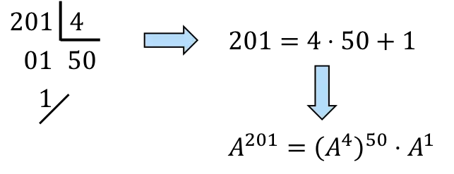

,然而,

将会是50次

还有一次


我们怎么知道
是单位矩阵


此外,将单位矩阵提升到任意数即可得到单位矩阵。然而:

最后,任何矩阵乘以单位矩阵都会得到相同的矩阵。所以:

为了什么
等于
![\displaystyle A^{201}= A =\begin{pmatrix} \bm{0} & \bm{-1} \\[1.1ex] \bm{1} & \bm{0} \end{pmatrix}](https://mathority.org/wp-content/ql-cache/quicklatex.com-1214abe876a5aede8fbbce79009d5dbc_l3.png "Rendered by QuickLaTeX.com")
练习5
考虑以下 3 阶矩阵:
![\displaystyle A=\begin{pmatrix} 3 & 4 & -1 \\[1.1ex] -2 & -3 & 1 \\[1.1ex] -2 & -3 & 0 \end{pmatrix}](https://mathority.org/wp-content/ql-cache/quicklatex.com-b8f3ba8b2d15b622f99774be05aa2620_l3.png "Rendered by QuickLaTeX.com")
计算:

显然,计算矩阵的幂
这是一个太大的计算,无法手动完成,因此矩阵幂必须遵循某种模式。在这种情况下,需要计算

为了知道它们遵循的顺序:
![\displaystyle A^2= A \cdot A = \begin{pmatrix}3 & 4 & -1 \\[1.1ex] -2 & -3 & 1 \\[1.1ex] -2 & -3 & 0 \end{pmatrix} \cdot \begin{pmatrix} 3 & 4 & -1 \\[1.1ex] -2 & -3 & 1 \\[1.1ex] -2 & -3 & 0 \end{pmatrix} = \begin{pmatrix} 3 & 3 & 1 \\[1.1ex] -2 & -2 & -1 \\[1.1ex] 0 & 1 & -1 \end{pmatrix}](https://mathority.org/wp-content/ql-cache/quicklatex.com-4032b55d68a5615911a5b7c997b05e6f_l3.png "Rendered by QuickLaTeX.com")
![\displaystyle A^3= A^2 \cdot A = \begin{pmatrix}3 & 3 & 1 \\[1.1ex] -2 & -2 & -1 \\[1.1ex] 0 & 1 & -1\end{pmatrix} \cdot \begin{pmatrix} 3 & 4 & -1 \\[1.1ex] -2 & -3 & 1 \\[1.1ex] -2 & -3 & 0 \end{pmatrix} = \begin{pmatrix} 1 & 0 & 0 \\[1.1ex] 0 & 1 & 0 \\[1.1ex] 0 & 0 & 1 \end{pmatrix}](https://mathority.org/wp-content/ql-cache/quicklatex.com-8b5deef2a7728c5e82e1a1dafb1a939c_l3.png "Rendered by QuickLaTeX.com")
![\displaystyle A^4= A^3 \cdot A = \begin{pmatrix}1 & 0 & 0 \\[1.1ex] 0 & 1 & 0 \\[1.1ex] 0 & 0 & 1 \end{pmatrix} \cdot \begin{pmatrix} 3 & 4 & -1 \\[1.1ex] -2 & -3 & 1 \\[1.1ex] -2 & -3 & 0 \end{pmatrix} = \begin{pmatrix} 3 & 4 & -1 \\[1.1ex] -2 & -3 & 1 \\[1.1ex] -2 & -3 & 0 \end{pmatrix}](https://mathority.org/wp-content/ql-cache/quicklatex.com-f62e856d037138b2ead39b17ccebf96d_l3.png "Rendered by QuickLaTeX.com")
![\displaystyle A^5= A^4 \cdot A = \begin{pmatrix}3 & 4 & -1 \\[1.1ex] -2 & -3 & 1 \\[1.1ex] -2 & -3 & 0 \end{pmatrix} \cdot \begin{pmatrix} 3 & 4 & -1 \\[1.1ex] -2 & -3 & 1 \\[1.1ex] -2 & -3 & 0 \end{pmatrix} = \begin{pmatrix} 3 & 3 & 1 \\[1.1ex] -2 & -2 & -1 \\[1.1ex] 0 & 1 & -1 \end{pmatrix}](https://mathority.org/wp-content/ql-cache/quicklatex.com-854da5c09b6662da46acb790afb6d01a_l3.png "Rendered by QuickLaTeX.com")
![\displaystyle A^6= A^5 \cdot A = \begin{pmatrix}3 & 3 & 1 \\[1.1ex] -2 & -2 & -1 \\[1.1ex] 0 & 1 & -1\end{pmatrix} \cdot \begin{pmatrix} 3 & 4 & -1 \\[1.1ex] -2 & -3 & 1 \\[1.1ex] -2 & -3 & 0 \end{pmatrix} = \begin{pmatrix} 1 & 0 & 0 \\[1.1ex] 0 & 1 & 0 \\[1.1ex] 0 & 0 & 1 \end{pmatrix}](https://mathority.org/wp-content/ql-cache/quicklatex.com-c9f804a1c129e18d105fb92254c971fa_l3.png "Rendered by QuickLaTeX.com")
通过这些计算我们可以看到每 3 次方我们就得到了单位矩阵。也就是说,它会给我们结果的幂单位矩阵

,

,

,
,…以便计算
我们必须将 62 分解为 3 的倍数:


,然而,
将会是20次

还有一次


我们怎么知道
是单位矩阵


此外,将单位矩阵提升到任意数即可得到单位矩阵。然而:

最后,任何矩阵乘以单位矩阵都会得到相同的矩阵。然而:

为了什么

将等于

,我们之前计算过的结果:
![\displaystyle A^{62}= A^2=\begin{pmatrix} \bm{3} & \bm{3} & \bm{1} \\[1.1ex] \bm{-2} & \bm{-2} & \bm{-1} \\[1.1ex] \bm{0} & \bm{1} & \bm{-1} \end{pmatrix}](https://mathority.org/wp-content/ql-cache/quicklatex.com-3f95e17aacde501ca1c28dbf14324f0b_l3.png "Rendered by QuickLaTeX.com")
如果这些关于方阵幂的练习对您有用,您还可以找到关于矩阵加法和减法(最常用的矩阵运算之一)的已解决分步练习。