在此页面上,您将找到什么是标量矩阵以及标量矩阵的几个示例,以便完全理解它。此外,您将能够看到标量矩阵的所有属性以及使用它们进行运算的优点。最后,我们解释如何计算标量矩阵的行列式以及如何反转此类矩阵。
什么是标量矩阵?
标量矩阵是对角矩阵,其中主对角线上的所有值都相等。
这是标量矩阵的定义,但我确信通过示例可以更好地理解它:😉
标量数组的示例
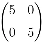
2×2 阶标量矩阵的示例
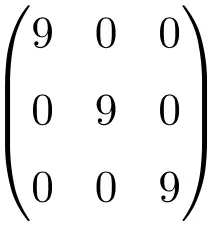
3×3 标量矩阵的示例
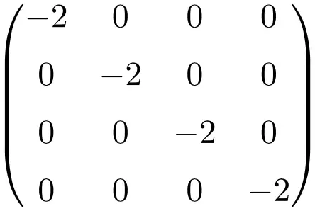
大小为 4×4 的标量矩阵的示例
标量矩阵的性质
标量矩阵也是一个对角矩阵,所以你会看到它继承了这个矩阵类的许多特性:
- 所有标量矩阵也是对称矩阵。
- 标量矩阵既是上三角矩阵又是下三角矩阵。
- 单位矩阵是标量矩阵。
- 任何标量矩阵都可以通过单位矩阵和标量数的乘积获得。
![4 \cdot \begin{pmatrix} 1 & 0 & 0 \\[1.1ex] 0 & 1 & 0 \\[1.1ex] 0 & 0 & 1 \end{pmatrix} = \begin{pmatrix} 4 & 0 & 0 \\[1.1ex] 0 & 4 & 0 \\[1.1ex] 0 & 0 & 4 \end{pmatrix}](https://mathority.org/wp-content/ql-cache/quicklatex.com-b77f7d177c2769b0847de258adfd1386_l3.png "Rendered by QuickLaTeX.com")
- 零矩阵也是标量矩阵。
- 标量矩阵的特征值(或特征值)是其主对角线的元素。因此,它们的特征值将始终相同,并且会重复与矩阵维数一样多的次数。
![\begin{pmatrix} 8 & 0 & 0 \\[1.1ex] 0 & 8 & 0 \\[1.1ex] 0 & 0 & 8 \end{pmatrix} \longrightarrow \ \lambda = 8 \ ; \ \lambda = 8 \ ; \ \lambda = 8](https://mathority.org/wp-content/ql-cache/quicklatex.com-2513b8d4aeb6d932d9870934102a1637_l3.png "Rendered by QuickLaTeX.com")
- 一个标量矩阵的伴随是另一个标量矩阵。而且,附加矩阵的主对角线的值将始终是原始矩阵的值提升到矩阵 – 1 的阶数。
![\displaystyle A=\begin{pmatrix} 5 & 0 & 0 \\[1.1ex] 0 & 5 & 0 \\[1.1ex] 0 & 0 & 5 \end{pmatrix} \longrightarrow \text{Adj}(A)=\begin{pmatrix} 5^{3-1} & 0 & 0 \\[1.1ex] 0 & 5^{3-1} & 0 \\[1.1ex] 0 & 0 & 5^{3-1} \end{pmatrix}= \begin{pmatrix} 25 & 0 & 0 \\[1.1ex] 0 & 25 & 0 \\[1.1ex] 0 & 0 & 25 \end{pmatrix}](https://mathority.org/wp-content/ql-cache/quicklatex.com-1f7e94cc5a528abace04016dc263c8f9_l3.png "Rendered by QuickLaTeX.com")
标量矩阵的运算
标量矩阵在线性代数中如此广泛使用的原因之一是它们允许您轻松地执行计算。这就是为什么它们在数学中如此重要。
那么让我们看看为什么使用这种类型的方阵进行计算如此容易:
标量矩阵的加法和减法
两个标量矩阵相加(或相减)非常简单:只需相加(或相减)主对角线上的数字即可。例如:
![\displaystyle \begin{pmatrix} 4 & 0 & 0 \\[1.1ex] 0 & 4 & 0 \\[1.1ex] 0 & 0 & 4 \end{pmatrix} +\begin{pmatrix} 3 & 0 & 0 \\[1.1ex] 0 & 3 & 0 \\[1.1ex] 0 & 0 & 3 \end{pmatrix} = \begin{pmatrix} 7& 0 & 0 \\[1.1ex] 0 & 7 & 0 \\[1.1ex] 0 & 0 & 7 \end{pmatrix}](https://mathority.org/wp-content/ql-cache/quicklatex.com-761de4b4c9bdbbc835b366b21d8cfc2d_l3.png "Rendered by QuickLaTeX.com")
标量矩阵乘法
与加法和减法类似,要求解两个标量矩阵之间的乘法或矩阵乘积,只需将它们之间的对角线元素相乘即可。例如:
![\displaystyle \begin{pmatrix} 2 & 0 & 0 \\[1.1ex] 0 & 2 & 0 \\[1.1ex] 0 & 0 & 2 \end{pmatrix} \cdot\begin{pmatrix} 6 & 0 & 0 \\[1.1ex] 0 & 6 & 0 \\[1.1ex] 0 & 0 & 6 \end{pmatrix} = \begin{pmatrix} 12 & 0 & 0 \\[1.1ex] 0 & 12 & 0 \\[1.1ex] 0 & 0 & 12 \end{pmatrix}](https://mathority.org/wp-content/ql-cache/quicklatex.com-d30acbf9c6ad31625f8253549e659b02_l3.png "Rendered by QuickLaTeX.com")
标量矩阵的幂
计算标量矩阵的幂也非常简单:您必须将对角线的每个元素提高到指数。例如:
 *** QuickLaTeX cannot compile formula:
\displaystyle\left. \begin{pmatrix} 2 & 0 & 0 \\[1.1ex] 0 & 2 & 0 \\[1.1ex] 0 & 0 & 2 \end{pmatrix}\right.^4=\begin{pmatrix} 2^ 4 & 0 & 0 \\[1.1ex] 0 & 2^

*** Error message:
Missing $ inserted.
leading text: \displaystyle
Missing { inserted.
leading text: \end{document}
\begin{pmatrix} on input line 9 ended by \end{document}.
leading text: \end{document}
Improper \prevdepth.
leading text: \end{document}
Missing $ inserted.
leading text: \end{document}
Missing } inserted.
leading text: \end{document}
Missing } inserted.
leading text: \end{document}
Missing \cr inserted.
leading text: \end{document}
Missing $ inserted.
leading text: \end{document}
You can't use `\end' in internal vertical mode.
leading text: \end{document}
\begin{pmatrix} on input line 9 ended by \end{document}.
leading text: \end{document}
Missing } inserted.
leading text: \end{document}
Missing \right. inserted.
leading text: \end{document}
& 0 \\[1.1ex] 0 & 0 & 2^4 \end{pmatrix}= \begin{pmatrix} 16 & 0 & 0 \\[1.1ex] 0 & 16 & 0 \\[1.1ex] 0 & 0 和 16 \end{pmatrix}

\displaystyle \begin{vmatrix} 7 & 0 & 0 \\[1.1ex] 0 & 7 & 0 \\[1.1ex] 0 & 0 & 7 \end{vmatrix} = 7 \cdot 7 \cdot 7 = \bm {343}

\displaystyle \begin{vmatrix} 7 & 0 & 0 \\[1.1ex] 0 & 7 & 0 \\[1.1ex] 0 & 0 & 7 \end{vmatrix} = 7^3= \bm{343}
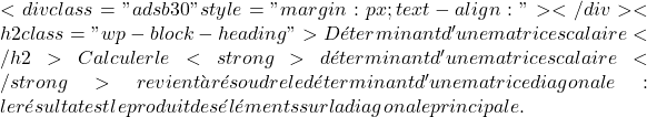
![Démontrer ce théorème est très simple : il suffit de calculer le déterminant d'une matrice scalaire par blocs (ou cofacteurs). Vous trouverez ci-dessous la <strong>démonstration</strong> de la formule utilisant une matrice scalaire générique :” title=”Rendered by QuickLaTeX.com” height=”62″ width=”1060″ style=”vertical-align: -4px;”></p>
<p> \begin{对齐} \begin{vmatrix} a & 0 & 0 \\[1.1ex] 0 & a & 0 \\[1.1ex] 0 & 0 & a \end{vmatrix}& = a \cdot \begin{ vmatrix} a & 0 \\[1.1ex] 0 & a \end{vmatrix} – 0 \cdot \begin{vmatrix} 0 & 0 \\[1.1ex] 0 & a \end{vmatrix} + 0 \cdot \开始{vmatrix} 0 & a \\[1.1ex] 0 & 0 \end{vmatrix} \\[2ex] & =a \cdot (a\cdot a) – 0 \cdot 0 + 0 \cdot 0 \\[ 2ex] & = a \cdot a \cdot a \\[2ex] & = a^3 \end{对齐}</p>
<p class=](https://mathority.org/wp-content/ql-cache/quicklatex.com-d24f9aa91fc9fe8ed74f705f83be3b32_l3.png)

一个^3
![car la matrice est d'ordre 3, mais il faut toujours l'élever à l'ordre de la matrice.
<div class="adsb30" style=" margin:12px; text-align:center">
<div id="ezoic-pub-ad-placeholder-118"></div>
</div>
<h2 class="wp-block-heading"> Inverser une matrice scalaire</h2>
<p> Une matrice scalaire <strong>est inversible si, et seulement si, tous les éléments de la diagonale principale sont différents de 0</strong> . Dans ce cas on dit que la matrice scalaire est une matrice régulière. De plus, l’inverse d’une matrice scalaire sera toujours une autre matrice scalaire avec les <strong>inverses</strong> de la diagonale principale :” title=”Rendered by QuickLaTeX.com” height=”174″ width=”1250″ style=”vertical-align: -5px;”></p>
<p> \displaystyle A= \begin{pmatrix} 9 & 0 & 0 \\[1.1ex] 0 & 9 & 0 \\[1.1ex] 0 & 0 & 9 \end{pmatrix} \ \longrightarrow \ A^{-1 }=\begin{pmatrix} \frac{1}{9} & 0 & 0 \\[1.1ex] 0 & \frac{1}{9} & 0 \\[1.1ex] 0 & 0 & \frac{ 1}{9} \end{pmatrix}</p>
<p class=](https://mathority.org/wp-content/ql-cache/quicklatex.com-49f5afdd3e1e9918f5323139662a2138_l3.png)

\displaystyle B= \begin{pmatrix} 2 & 0 & 0 \\[1.1ex] 0 & 2 & 0 \\[1.1ex] 0 & 0 & 2 \end{pmatrix} \displaystyle\left| B^{-1}\right|=\cfrac{1}{2} \cdot \cfrac{1}{2} \cdot \cfrac{1}{2}=\cfrac{1}{8} = $0.125