Multiplication d'un nombre par une matrice

Sur cette page nous allons voir comment multiplier un nombre par une matrice. Vous avez également des exemples qui vous aideront à le comprendre parfaitement et des exercices résolus pour que vous puissiez vous entraîner. Vous trouverez également toutes les propriétés du produit d’un scalaire et d’une matrice.

Comment faire une multiplication d’un nombre par une matrice ?

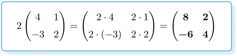
Pour multiplier un nombre par une matrice , multipliez chaque élément de la matrice par le nombre.

Exemple:

Problèmes résolus de multiplication d’un nombre par une matrice

Exercice 1 :

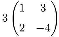
Exercice résolu du produit d'un nombre par une matrice 2x2, opérations avec des matrices

voir solution

C’est une multiplication d’un scalaire par une matrice carrée d’ordre 2 :

$\displaystyle 3 \begin{pmatrix} 1 & 3 \\[1.1ex] 2 & -4 \end{pmatrix} = \begin{pmatrix} 3\cdot 1 & 3\cdot 3 \\[1.1ex] 3\cdot 2 & 3\cdot (-4) \end{pmatrix} = \begin{pmatrix} \bm{3} & \bm{9} \\[1.1ex] \bm{6} & \bm{-12} \end{pmatrix}$

Exercice 2 :

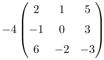
exercice résolu pas à pas de multiplication d'un nombre par une matrice 3x3, opérations avec des matrices

voir solution

C’est un produit d’un nombre par une matrice carrée d’ordre 3 :

$\displaystyle -4 \begin{pmatrix} 2 & 1 & 5 \\[1.1ex] -1 & 0 & 3 \\[1.1ex] 6 & -2 & -3 \end{pmatrix} = \begin{pmatrix} -4 \cdot 2 & -4 \cdot 1 & -4 \cdot 5 \\[1.1ex] -4 \cdot (-1) & -4 \cdot 0 & -4 \cdot 3 \\[1.1ex] -4 \cdot 6 & -4 \cdot (-2) & -4 \cdot (-3) \end{pmatrix}= \begin{pmatrix} \bm{-8} & \bm{-4} & \bm{-20} \\[1.1ex] \bm{4} & \bm{0} & \bm {-12} \\[1.1ex] \bm{-24} & \bm{8} & \bm {12} \end{pmatrix}$

Exercice 3 :

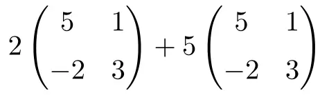
Exercice résolu de multiplication d'un nombre par une matrice 2x2, opérations combinées avec des matrices

voir solution

C’est une opération qui combine des produits de nombres par des matrices et des sommes de matrices de dimension 2×2 :

$\displaystyle 2 \begin{pmatrix} 5 & 1 \\[1.1ex] -2 & 3 \end{pmatrix}+5\begin{pmatrix} 5 & 1 \\[1.1ex] -2 & 3 \end{pmatrix}$

Par conséquent, nous devons d’abord résoudre pour les produits:

$\displaystyle \begin{pmatrix} 10 & 2 \\[1.1ex] -4 & 6 \end{pmatrix}+\begin{pmatrix} 25 & 5 \\[1.1ex] -10 & 15 \end{pmatrix}$

Et enfin on fait la somme des matrices résultantes :

$\displaystyle \begin{pmatrix} \bm{35} & \bm{7} \\[1.1ex] \bm{-14} & \bm{21} \end{pmatrix}$

Exercice 4 :

Soit les matrices suivantes :

$\displaystyle A=\begin{pmatrix} 2 & -3 & 5 \\ 1 & 4 & 0 \\ -3 & 2 & -5 \end{pmatrix} \qquad B=\begin{pmatrix} 6 & 0 & 2 \\ -3 & 4 & 1 \\ 3 & 2 & 7 \end{pmatrix}$

Calculer:

$\displaystyle -2A+5I-3B$

voir solution

C’est une opération qui combine des multiplications scalaires avec des additions et des soustractions de matrices de dimension 3×3. De plus, la matrice

$I$ est la matrice identité, qui est composée de 1 sur la diagonale principale et de 0 sur le reste des éléments :

$\displaystyle -2\begin{pmatrix} 2 & -3 & 5 \\[1.1ex] 1 & 4 & 0 \\[1.1ex] -3 & 2 & -5 \end{pmatrix}+5\begin{pmatrix} 1 & 0 & 0 \\[1.1ex] 0 & 1 & 0 \\[1.1ex] 0 & 0 & 1 \end{pmatrix} -3 \begin{pmatrix} 6 & 0 & 2 \\[1.1ex] -3 & 4 & 1 \\[1.1ex] 3 & 2 & 7 \end{pmatrix}$

Par conséquent, nous effectuons d’abord les multiplications :

$\displaystyle \begin{pmatrix} -4 & 6 & -10 \\[1.1ex] -2 & -8 & 0 \\[1.1ex] 6 & -4 & 10 \end{pmatrix}+\begin{pmatrix} 5 & 0 & 0 \\[1.1ex] 0 & 5 & 0 \\[1.1ex] 0 & 0 & 5 \end{pmatrix} - \begin{pmatrix} 18 & 0 & 6 \\[1.1ex] -9 & 12 & 3 \\[1.1ex] 9 & 6 & 21 \end{pmatrix}$

On additionne les deux premières matrices :

$\displaystyle \begin{pmatrix} 1 & 6 & -10 \\[1.1ex] -2 & -3 & 0 \\[1.1ex] 6 & -4 & 15 \end{pmatrix}-\begin{pmatrix} 18 & 0 & 6 \\[1.1ex] -9 & 12 & 3 \\[1.1ex] 9 & 6 & 21 \end{pmatrix}$

Enfin, on effectue la soustraction des matrices :

$\displaystyle \begin{pmatrix} \bm{-17} & \bm{6} & \bm{-16} \\[1.1ex] \bm{7} & \bm{-15} & \bm{-3} \\[1.1ex] \bm{-3} & \bm{-10} & \bm{-6} \end{pmatrix}$

Si ces exercices sur les produits scalaires matriciels vous ont été utiles, n’hésitez pas à vous exercer avec les exercices résolus pas à pas sur l’ addition de matrices et le produit de matrices , les deux types d’opérations matricielles qui se répètent le plus.

Propriétés du produit d’un nombre par une matrice

Comme vous le savez bien, il existe de nombreux types de matrices : les matrices carrées, les matrices triangulaires, la matrice identité,… Mais, heureusement, toutes les propriétés du produit de nombres par des matrices sont valables pour toutes les classes de matrices.

Voici donc les propriétés de la multiplication entre scalaires et matrices :

Propriété associative :

$a \cdot (b \cdot A) = (a \cdot b) \cdot A$

Regardez les deux opérations suivantes car elles donnent le même résultat, quelle que soit la façon dont nous multiplions le 2 et le 3 :

$\displaystyle 2 \cdot \left(3 \cdot \begin{pmatrix} 1 & 0 \\[1.1ex] 2 & -1 \end{pmatrix} \right) =2 \cdot \begin{pmatrix} 3 & 0 \\[1.1ex] 6 & -3 \end{pmatrix} = \begin{pmatrix} \bm{6} & \bm{0} \\[1.1ex] \bm{12} & \bm{-6} \end{pmatrix}$

$\displaystyle (2 \cdot 3) \cdot \begin{pmatrix} 1 & 0 \\[1.1ex] 2 & -1 \end{pmatrix} =6 \cdot \begin{pmatrix} 1 & 0 \\[1.1ex] 2 & -1 \end{pmatrix} = \begin{pmatrix} \bm{6} & \bm{0} \\[1.1ex] \bm{12} & \bm{-6} \end{pmatrix}$

Propriété distributive par rapport à l’addition de scalaires :

$(a+b) \cdot A = a \cdot A+ b \cdot A$

Comme vous pouvez le voir dans l’exemple ci-dessous, il en va de même si nous additionnons d’abord 1+2 puis le multiplions par une matrice, ou si nous multiplions la matrice séparément par 1 et par 2 puis additionnons les résultats :

$\displaystyle (1 + 2) \cdot \begin{pmatrix} 2 & -1 \\[1.1ex] 3 & 5 \\[1.1ex] -2 & -4 \end{pmatrix} =3 \cdot \begin{pmatrix} 2 & -1 \\[1.1ex] 3 & 5 \\[1.1ex] -2 & -4 \end{pmatrix}= \begin{pmatrix} \bm{6} & \bm{-3} \\[1.1ex] \bm{9} & \bm{15} \\[1.1ex] \bm{-6} & \bm{-12} \end{pmatrix}$

$\displaystyle 1 \cdot \begin{pmatrix} 2 & -1 \\[1.1ex] 3 & 5 \\[1.1ex] -2 & -4 \end{pmatrix} + 2 \cdot \begin{pmatrix} 2 & -1 \\[1.1ex] 3 & 5 \\[1.1ex] -2 & -4\end{pmatrix} = \begin{pmatrix} 2 & -1 \\[1.1ex] 3 & 5\\[1.1ex] -2 & -4 \end{pmatrix} + \begin{pmatrix} 4 & -2 \\[1.1ex] 6 & 10 \\[1.1ex] -4 & -8\end{pmatrix}= \begin{pmatrix} \bm{6} & \bm{-3} \\[1.1ex] \bm{9} & \bm{15} \\[1.1ex] \bm{-6} & \bm{-12} \end{pmatrix}$

Propriété distributive par rapport à l’addition de matrices :

$a \cdot \left(A + B \right) = a \cdot A + a \cdot B$

Autrement dit, ajouter deux matrices mathématiques puis les multiplier par un nombre équivaut à multiplier séparément les deux matrices par le même nombre puis à additionner les résultats. Dans l’exemple ci-dessous, vous pouvez vérifier :

$\displaystyle 4 \cdot \left( \begin{pmatrix} 3 & -2 \\[1.1ex] 6 & -1 \end{pmatrix}+\begin{pmatrix} -1 & 3 \\[1.1ex] 0 & 4 \end{pmatrix} \right) =4 \cdot \begin{pmatrix} 2 & 1 \\[1.1ex] 6 & 3 \end{pmatrix}= \begin{pmatrix} \bm{8} & \bm{4} \\[1.1ex] \bm{24} & \bm{12} \end{pmatrix}$

$\displaystyle 4 \cdot \begin{pmatrix} 3 & -2 \\[1.1ex] 6 & -1 \end{pmatrix}+ 4 \cdot \begin{pmatrix} -1 & 3 \\[1.1ex] 0 & 4 \end{pmatrix} = \begin{pmatrix} 12 & -8 \\[1.1ex] 24 & -4 \end{pmatrix}+\begin{pmatrix} -4 & 12 \\[1.1ex] 0 & 16 \end{pmatrix} = \begin{pmatrix} \bm{8} & \bm{4} \\[1.1ex] \bm{24} & \bm{12} \end{pmatrix}$

Propriété de l’élément neutre :

$1 \cdot A = A$

Par conséquent, en multipliant une matrice par 1, nous ne modifions pas la matrice :

$\displaystyle 1 \cdot \begin{pmatrix} 5 & -4 & 0 \\[1.1ex] 1 & 3 & -3 \\[1.1ex] 2 & 9 & 4 \end{pmatrix}=\begin{pmatrix} \bm{5} & \bm{-4} & \bm{0} \\[1.1ex] \bm{1} & \bm{3} & \bm{-3} \\[1.1ex] \bm{2} & \bm{9} & \bm{4} \end{pmatrix}$

Ce sont toutes les propriétés du produit d’un scalaire et d’une matrice, c’est donc la fin de cet article. Nous espérons que cela vous a plu et, surtout, que vous avez appris à résoudre la multiplication de nombres avec des matrices.

Par contre, d’autres opérations matricielles liées à la multiplication, et qui sont très utiles, sont les puissances. Ici, nous vous laissons la page où vous apprendrez ce que c’est et comment résoudre la puissance d’une matrice , au cas où vous seriez curieux.

Multiplication d’un nombre par une matrice

Comment faire une multiplication d’un nombre par une matrice ?

Exemple:

Problèmes résolus de multiplication d’un nombre par une matrice

Exercice 1 :

Exercice 2 :

Exercice 3 :

Exercice 4 :

Propriétés du produit d’un nombre par une matrice

Leave a Comment Cancel Reply