Multiplication matricielle

Sur cette page nous allons voir comment faire une multiplication de matrices de dimension 2×2, 3×3, 4×4, etc. Nous expliquons pas à pas la procédure de multiplication des matrices à travers un exemple, puis vous trouverez des exercices résolus pour que vous puissiez également vous entraîner. Enfin, vous apprendrez quand deux matrices ne peuvent pas être multipliées et toutes les propriétés de cette opération matricielle.

Comment multiplier deux matrices ?

Voyons la procédure pour effectuer la multiplication de deux matrices avec un exemple :

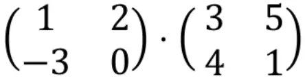
Pour calculer une multiplication matricielle, les lignes de la matrice de gauche doivent être multipliées par les colonnes de la matrice de droite.

Nous devons donc d’abord multiplier la première ligne par la première colonne. Pour ce faire, nous multiplions un par un chaque élément de la première ligne par chaque élément de la première colonne, et additionnons les résultats. Donc tout cela sera le premier élément de la première ligne du tableau résultant. Regarde la procédure :

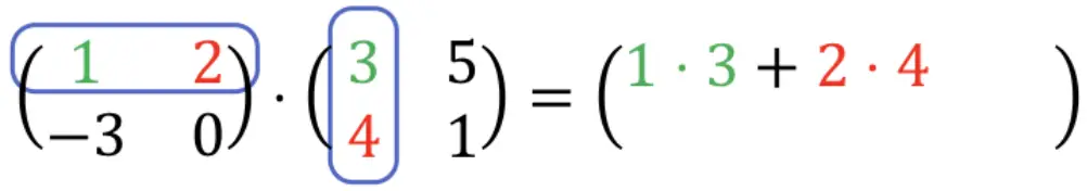
comment résoudre une multiplication matricielle 2x2, opérations avec des matrices

1 ⋅ 3 + 2 ⋅ 4 = 3 + 8 = 11. Donc :

Maintenant, nous devons multiplier la première ligne par la deuxième colonne . On répète donc la procédure : on multiplie un par un chaque élément de la première ligne par chaque élément de la deuxième colonne, et on additionne les résultats. Et tout cela sera le deuxième élément de la première ligne du tableau résultant :

1 ⋅ 5 + 2 ⋅ 1 = 5 + 2 = 7. Donc :

Une fois que nous avons rempli la première ligne de la matrice résultante, nous passons à la deuxième ligne. Nous multiplions donc la deuxième ligne par la première colonne en répétant la procédure : nous multiplions un par un chaque élément de la deuxième ligne par chaque élément de la première colonne, et additionnons les résultats :

-3 ⋅ 3 + 0 ⋅ 4 = -9 + 0 = -9. Pourtant:

Enfin, nous multiplions la deuxième ligne par la deuxième colonne . Toujours avec la même procédure : on multiplie un par un chaque élément de la deuxième ligne par chaque élément de la deuxième colonne, et on additionne les résultats :

-3 ⋅ 5 + 0 ⋅ 1 = -15 + 0 = -15. Pourtant:

Et ici se termine la multiplication des deux matrices. Comme vous l’avez vu, vous devez multiplier les lignes par les colonnes, en répétant toujours la même procédure : multipliez chaque élément de la ligne par chaque élément de la colonne un par un, et additionnez les résultats.

Exercices résolus de multiplications matricielles

Exercice 1

Résolvez le produit matriciel suivant :

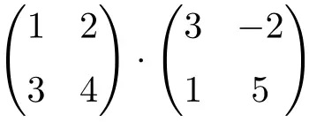
exercice résolu pas à pas de produit de matrices 2x2, opérations avec des matrices

voir solution

C’est un produit de matrices d’ordre 2 :

$\displaystyle \begin{pmatrix} 1 & 2 \\[1.1ex] 3 & 4 \end{pmatrix} \cdot \begin{pmatrix} 3 & -2 \\[1.1ex] 1 & 5 \end{pmatrix}$

Pour résoudre un produit matriciel, il faut multiplier les lignes de la matrice de gauche par les colonnes de la matrice de droite.

Nous multiplions donc d’abord la première ligne par la première colonne. Pour ce faire, nous multiplions un par un chaque élément de la première ligne par chaque élément de la première colonne, et additionnons les résultats. Et tout cela sera le premier élément de la première ligne du tableau résultant :

$\displaystyle \begin{pmatrix} 1 & 2 \\[1.1ex] 3 & 4 \end{pmatrix} \cdot \begin{pmatrix} 3 & -2 \\[1.1ex] 1 & 5 \end{pmatrix} = \begin{pmatrix} 1\cdot 3 +2 \cdot 1 & \\[1.1ex] & \end{pmatrix} = \begin{pmatrix} 5 & \\[1.1ex] & \end{pmatrix}$

Multiplions maintenant la première ligne par la deuxième colonne, pour obtenir le deuxième élément de la première ligne de la matrice résultante :

$\displaystyle \begin{pmatrix} 1 & 2 \\[1.1ex] 3 & 4 \end{pmatrix} \cdot \begin{pmatrix} 3 & -2 \\[1.1ex] 1 & 5 \end{pmatrix} = \begin{pmatrix} -1 & 1\cdot (-2) +2 \cdot 5 \\[1.1ex] & \end{pmatrix} = \begin{pmatrix}5 & 8 \\[1.1ex] & \end{pmatrix}$

Nous allons à la deuxième ligne, donc, nous multiplions la deuxième ligne par la première colonne :

$\displaystyle \begin{pmatrix} 1 & 2 \\[1.1ex] 3 & 4 \end{pmatrix} \cdot \begin{pmatrix} 3 & -2 \\[1.1ex] 1 & 5 \end{pmatrix} = \begin{pmatrix} -1 & 8 \\[1.1ex] 3\cdot 3 +4 \cdot 1 & \end{pmatrix}= \begin{pmatrix}5 & 8 \\[1.1ex] 13 & \end{pmatrix}$

Enfin, on multiplie la seconde ligne par la seconde colonne , pour calculer le dernier élément du tableau :

$\displaystyle \begin{pmatrix} 1 & 2 \\[1.1ex] 3 & 4 \end{pmatrix} \cdot \begin{pmatrix} 3 & -2 \\[1.1ex] 1 & 5 \end{pmatrix}= \begin{pmatrix} -1 & 8 \\[1.1ex]1 & 3\cdot (-2) +4 \cdot 5 \end{pmatrix}=\begin{pmatrix} 5 & 8 \\[1.1ex] 13 & 14 \end{pmatrix}$

Donc le résultat de la multiplication matricielle est :

$\displaystyle \begin{pmatrix} \bm{5} & \bm{8} \\[1.1ex]\bm{13} & \bm{14} \end{pmatrix}$

Exercice 2

Trouvez le résultat de la multiplication matricielle carrée 2×2 suivante :

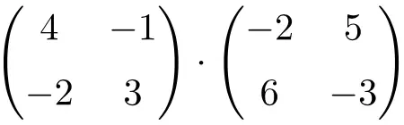
Exercice résolu pas à pas de multiplication matricielle 2x2, opérations matricielles

voir solution

C’est un produit de matrices de dimension 2×2.

Pour résoudre la multiplication, il faut multiplier les lignes de la matrice de gauche par les colonnes de la matrice de droite :

$\displaystyle \begin{aligned} \begin{pmatrix} 4 & -1 \\[1.1ex] -2 & 3 \end{pmatrix} \cdot \begin{pmatrix} -2 & 5 \\[1.1ex] 6 & -3 \end{pmatrix} & = \begin{pmatrix} 4\cdot (-2)+(-1) \cdot 6 & 4\cdot 5+(-1) \cdot (-3) \\[1.1ex](-2)\cdot (-2)+3 \cdot 6 & (-2)\cdot 5+3 \cdot (-3)\end{pmatrix} \\[2ex] & =\begin{pmatrix} \bm{-14} & \bm{23} \\[1.1ex]\bm{22} & \bm{-19} \end{pmatrix} \end{aligned}$

Exercice 3

Calculez la multiplication matricielle 3×3 suivante :

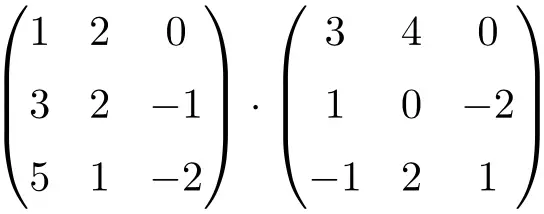
exercice résolu pas à pas de multiplication de matrices 3x3, opérations de matrices

voir solution

Pour faire la multiplication matricielle 3×3, il faut multiplier les lignes de la matrice de gauche par les colonnes de la matrice de droite :

$\displaystyle \begin{array}{l} \begin{pmatrix} 1 & 2 & 0 \\[1.1ex] 3 & 2 & -1 \\[1.1ex] 5 & 1 & -2 \end{pmatrix} \cdot \begin{pmatrix} 3 & 4 & 0 \\[1.1ex] 1 & 0 & -2 \\[1.1ex] -1 & 2 & 1 \end{pmatrix} = \\[7.5ex] =\begin{pmatrix} 1 \cdot 3+2 \cdot 1+ 0 \cdot (-1) & 1 \cdot 4+2 \cdot 0+ 0 \cdot 2 & 1 \cdot 0+2 \cdot (-2)+ 0 \cdot 1 \\[1.1ex] 3 \cdot 3+2 \cdot 1+ (-1) \cdot (-1) & 3 \cdot 4+2 \cdot 0+ (-1) \cdot 2 & 3 \cdot 0+2 \cdot (-2)+ (-1) \cdot 1 \\[1.1ex] 5 \cdot 3+1 \cdot 1+ (-2) \cdot (-1) & 5 \cdot 4+1 \cdot 0+ (-2) \cdot 2 & 5 \cdot 0+1 \cdot (-2)+ (-2) \cdot 1 \end{pmatrix} = \\[7.5ex] =\begin{pmatrix} \bm{5} & \bm{4} & \bm{-4} \\[1.1ex] \bm{12} & \bm{10} & \bm{-5} \\[1.1ex] \bm{18} & \bm{16} & \bm{-4} \end{pmatrix}\end{array}$

Exercice 4

étant donné la matrice

$A$ :

$\displaystyle A= \begin{pmatrix} 3 & 1 & -2 \\[1.1ex] 4 & 2 & -1 \end{pmatrix}$

Calculer:

$\displaystyle 2A\cdot A^t$

voir solution

Nous allons d’abord calculer la matrice transposée de

$A$ pour faire la multiplication. Et pour faire la matrice transposée, nous devons changer les lignes en colonnes. Autrement dit, la première ligne de la matrice devient la première colonne de la matrice et la deuxième ligne de la matrice devient la deuxième colonne de la matrice. Pourtant:

$\displaystyle A^t= \begin{pmatrix} 3 & 4 \\[1.1ex] 1 & 2 \\[1.1ex] -2 & -1 \end{pmatrix}$

L’opération matricielle reste donc :

$\displaystyle 2A\cdot A^t = 2 \begin{pmatrix} 3 & 1 & -2 \\[1.1ex] 4 & 2 & -1 \end{pmatrix} \cdot \begin{pmatrix} 3 & 4 \\[1.1ex] 1 & 2 \\[1.1ex] -2 & -1 \end{pmatrix}$

Maintenant, nous pouvons faire les calculs. On calcule d’abord

$2A$ (bien qu’on puisse aussi d’abord calculer $A \cdot A^t$ ):

$\displaystyle \begin{pmatrix} 2 \cdot 3 & 2 \cdot 1 & 2 \cdot (-2) \\[1.1ex] 2 \cdot 4 & 2 \cdot 2 & 2 \cdot (-1) \end{pmatrix} \cdot \begin{pmatrix} 3 & 4 \\[1.1ex] 1 & 2 \\[1.1ex] -2 & -1 \end{pmatrix} =$

$\displaystyle =\begin{pmatrix} 6 & 2 & -4 \\[1.1ex] 8 & 4 & -2 \end{pmatrix} \cdot \begin{pmatrix} 3 & 4 \\[1.1ex] 1 & 2 \\[1.1ex] -2 & -1 \end{pmatrix}$

Et, enfin, on résout le produit de matrices :

$\displaystyle \begin{pmatrix} 6 \cdot 3 +2 \cdot 1 + (-4) \cdot (-2) & 6 \cdot 4 +2 \cdot 2 + (-4) \cdot (-1) \\[1.1ex] 8 \cdot 3 +4 \cdot 1 + (-2) \cdot (-2) & 8 \cdot 4 +4 \cdot 2 + (-2) \cdot (-1) \end{pmatrix} =$

$\displaystyle = \begin{pmatrix} \bm{28} & \bm{32} \\[1.1ex]\bm{32} & \bm{42} \end{pmatrix}$

Exercice 5

Soit les matrices suivantes :

$\displaystyle A=\begin{pmatrix} 2 & 4 \\[1.1ex] -3 & 5 \end{pmatrix} \qquad B=\begin{pmatrix} -1 & -2 \\[1.1ex] 3 & -3 \end{pmatrix}$

Calculer:

$\displaystyle A\cdot B - B \cdot A$

voir solution

C’est une opération qui combine la soustraction avec des multiplications matricielles d’ordre 2 :

$\displaystyle A\cdot B - B \cdot A= \begin{pmatrix} 2 & 4 \\[1.1ex] -3 & 5 \end{pmatrix}\cdot \begin{pmatrix} -1 & -2 \\[1.1ex] 3 & -3 \end{pmatrix} - \begin{pmatrix} -1 & -2 \\[1.1ex] 3 & -3 \end{pmatrix} \cdot \begin{pmatrix} 2 & 4 \\[1.1ex] -3 & 5 \end{pmatrix}$

On calcule d’abord la multiplication à gauche :

$\displaystyle \begin{pmatrix} 2\cdot (-1) + 4 \cdot 3 & 2\cdot (-2) + 4 \cdot (-3) \\[1.1ex] (-3)\cdot (-1) + 5 \cdot 3 & (-3)\cdot (-2) + 5 \cdot (-3) \end{pmatrix} - \begin{pmatrix} -1 & -2 \\[1.1ex] 3 & -3 \end{pmatrix} \cdot \begin{pmatrix} 2 & 4 \\[1.1ex] -3 & 5 \end{pmatrix} =$

$\displaystyle= \begin{pmatrix} 10 & -16 \\[1.1ex] 18 & -9 \end{pmatrix} - \begin{pmatrix} -1 & -2 \\[1.1ex] 3 & -3 \end{pmatrix} \cdot \begin{pmatrix} 2 & 4 \\[1.1ex] -3 & 5 \end{pmatrix}$

Maintenant, nous résolvons la multiplication à droite :

$\displaystyle \begin{pmatrix} 10 & -16 \\[1.1ex] 18 & -9 \end{pmatrix} - \begin{pmatrix} -1 \cdot 2 +(-2) \cdot (-3) & -1 \cdot 4 +(-2) \cdot 5 \\[1.1ex]3 \cdot 2 +(-3) \cdot (-3) & 3 \cdot 4 +(-3) \cdot 5 \end{pmatrix} =$

$\displaystyle =\begin{pmatrix} 10 & -16 \\[1.1ex] 18 & -9 \end{pmatrix} - \begin{pmatrix} 4 &-14 \\[1.1ex]15 & -3 \end{pmatrix}$

Et enfin on soustrait les matrices :

$\displaystyle \begin{pmatrix} 10-4 & -16 -(-14) \\[1.1ex] 18-15 & -9-(-3) \end{pmatrix} =$

$\displaystyle =\begin{pmatrix} \bm{6} & \bm{-2} \\[1.1ex] \bm{3} & \bm{-6} \end{pmatrix}$

Quand ne pouvez-vous pas multiplier deux matrices ?

Toutes les matrices ne peuvent pas être multipliées. Pour multiplier deux matrices, le nombre de colonnes de la première matrice doit correspondre au nombre de lignes de la seconde matrice.

Par exemple, la multiplication suivante ne peut pas être effectuée car la première matrice a 3 colonnes et la deuxième matrice a 2 lignes :

$\displaystyle\begin{pmatrix} 1 & 3 & -2 \\[1.1ex] 4 & 0 & 5 \end{pmatrix} \cdot \begin{pmatrix} 2 & 1 \\[1.1ex] 3 & -1 \end{pmatrix} \ \longleftarrow \ \color{red} \bm{\times}$

Mais si on inverse l’ordre, ils peuvent être multipliés. Parce que la première matrice a deux colonnes et la deuxième matrice a deux lignes :

$\displaystyle \begin{aligned} \begin{pmatrix} 2 & 1 \\[1.1ex] 3 & -1 \end{pmatrix} \cdot \begin{pmatrix} 1 & 3 & -2 \\[1.1ex] 4 & 0 & 5 \end{pmatrix} & = \begin{pmatrix} 2\cdot 1 + 1 \cdot 4 & 2\cdot 3 + 1 \cdot 0 & 2\cdot (-2) + 1 \cdot 5 \\[1.1ex] 3\cdot 1 + (-1) \cdot 4 & 3\cdot 3 + (-1) \cdot 0 & 3\cdot (-2) + (-1) \cdot 5 \end{pmatrix} \\[2ex] & = \begin{pmatrix} \bm{6} & \bm{6} & \bm{1} \\[1.1ex]\bm{-1} & \bm{9} & \bm{-11} \end{pmatrix} \end{aligned}$

Propriétés de multiplication matricielle

Ce type d’opération matricielle a les caractéristiques suivantes :

La multiplication matricielle est associative :

$\displaystyle \left( A \cdot B \right) \cdot C = A \cdot \left( B \cdot C \right)$

La multiplication matricielle a également la propriété distributive :

$\displaystyle A\cdot \left(B+C\right) = A\cdot B + A \cdot C$

Le produit des matrices n’est pas commutatif :

$\displaystyle A \cdot B \neq B \cdot A$

Par exemple, la multiplication matricielle suivante donne un résultat :

$\displaystyle \begin{aligned} \begin{pmatrix} 1 & -1 \\[1.1ex] 2 & 3 \end{pmatrix} \cdot \begin{pmatrix} -2 & 5 \\[1.1ex] 0 & 1 \end{pmatrix} & = \begin{pmatrix} 1\cdot (-2) + (-1) \cdot 0 & 1\cdot 5 + (-1) \cdot 1 \\[1.1ex] 2\cdot (-2) + 3 \cdot 0 & 2\cdot 5 + 3 \cdot 1 \end{pmatrix} \\[2ex] & = \begin{pmatrix} \bm{-2} & \bm{4} \\[1.1ex] \bm{-4} & \bm{13} \end{pmatrix}\end{aligned}$

Mais le résultat du produit est différent si on inverse l’ordre de multiplication des matrices :

$\displaystyle \begin{aligned}\begin{pmatrix} -2 & 5 \\[1.1ex] 0 & 1 \end{pmatrix} \cdot \begin{pmatrix} 1 & -1 \\[1.1ex] 2 & 3 \end{pmatrix} & = \begin{pmatrix} -2 \cdot 1 + 5\cdot 2 & -2 \cdot (-1) + 5\cdot 3 \\[1.1ex] 0 \cdot 1 + 1\cdot 2 & 0 \cdot (-1) + 1\cdot 3 \end{pmatrix} \\[2ex] & = \begin{pmatrix} \bm{8} & \bm{17} \\[1.1ex] \bm{2} & \bm{3} \end{pmatrix}\end{aligned}$

De plus, toute matrice multipliée par la matrice d’identité donne la même matrice. C’est ce qu’on appelle la propriété d’identité multiplicative :

$\displaystyle A \cdot I=A$

$\displaystyle I \cdot A=A$

Par exemple:

$\displaystyle \begin{pmatrix} 2 & 7 \\[1.1ex] -6 & 5 \end{pmatrix} \cdot \begin{pmatrix} 1 & 0 \\[1.1ex] 0 & 1 \end{pmatrix} = \begin{pmatrix} \bm{2} & \bm{7} \\[1.1ex] \bm{-6} & \bm{5} \end{pmatrix}$

Enfin, comme vous le devinez peut-être déjà, toute matrice multipliée par la matrice nulle est égale à la matrice nulle. C’est ce qu’on appelle la propriété multiplicative de zéro :

$\displaystyle A \cdot 0=0$

$\displaystyle 0\cdot A=0$

Par exemple:

$\displaystyle \begin{pmatrix} 6 & -4 \\[1.1ex] 3 & 8 \end{pmatrix} \cdot \begin{pmatrix} 0 & 0 \\[1.1ex] 0 & 0 \end{pmatrix} = \begin{pmatrix} \bm{0} & \bm{0} \\[1.1ex] \bm{0} & \bm{0}\end{pmatrix}$

Comment multiplier deux matrices ?

Exercices résolus de multiplications matricielles

Exercice 1

Exercice 2

Exercice 3

Exercice 4

Exercice 5

Quand ne pouvez-vous pas multiplier deux matrices ?

Propriétés de multiplication matricielle

Leave a Comment Cancel Reply